Optimal Control for Quantum Processors

Short Definition

Optimal control for a quantum processor is the engineering process that turns a physical target into a constrained search problem, chooses a search method compatible with the available model and experimental budget, and qualifies the resulting control artifact on the device where it will run. The artifact may be a sampled waveform, a compact analytic pulse, a sequence of primitive operations, or a policy whose next action depends on observations.

This page owns method selection, software integration, hardware-in-the-loop optimization, and deployment evidence. The canonical mathematical treatment of control dynamics, objective functionals, adjoint gradients, GRAPE, Krotov updates, and robustness ensembles is Optimal Control. Pulse-Level Control owns the executable waveform and delivery contract, while Calibration Loops owns scheduling, dependency invalidation, acceptance, publication, and rollback. Those boundaries matter: an optimizer proposes a candidate; it does not grant that candidate permission to become the active gate.

The method names alone say little about whether a result is trustworthy. GRAPE can optimize the wrong model very efficiently. CRAB can search a useful hardware-compatible family or an inadequate one. Reinforcement learning can represent an observation-dependent policy, but it can also consume an unacceptable number of experiments or exploit defects in a reward proxy. The right question is therefore not “Which optimizer is best?” but:

What information, action space, evaluation budget, and validation evidence does this control problem actually provide?

Three Distinct Deployment Regimes

The phrase closed-loop control is used for several different workflows. They should be separated before choosing an algorithm.

Regime	Information used during execution	Typical output	Optimization location
open-loop pulse design	time and a fixed initial condition	waveform or pulse parameters	simulation, then optional device refinement
hardware-in-the-loop tuning	repeated terminal measurements across experiments	updated fixed waveform or parameters	host or calibration service
measurement-based feedback	observations arriving within one experimental trajectory	causal policy or conditional pulse sequence	controller, FPGA, or tightly coupled host

An optimizer that repeatedly measures the device while tuning a fixed pulse is closed around a calibration loop, but the deployed pulse is still open-loop. In true measurement-based feedback, action $a_t$ depends causally on an observation history $o_{leq t}$ during the same run. This distinction changes the mathematical object being optimized, the latency budget, and the evidence required for deployment.

A fourth pattern, common in practice, is hybrid optimization: use a model to produce a strong initial candidate and then refine a small number of parameters using hardware measurements. This can reduce model bias without paying the experimental cost of searching an unrestricted waveform from scratch.

The Optimization Contract

Before selecting software, write down a typed optimization contract

$$\mathfrak C = \left( \mathcal T, \mathcal M, \mathcal A, \mathcal J, \mathcal K, p(\theta), \mathcal B, \mathcal V \right).$$

Its fields are:

• $\mathcal T$: the target state, unitary, channel, observable, or feedback behavior;
• $\mathcal M$: the dynamical and measurement model, including frame and dissipation conventions;
• $\mathcal A$: the admissible control representation and its parameter domain;
• $\mathcal J$: the physical objective and any surrogate used to estimate it;
• $\mathcal K$: hard constraints and soft penalties;
• $p(\theta)$: uncertainty over device, noise, and transfer-chain parameters;
• $\mathcal B$: computational, experimental, and wall-clock budgets;
• $\mathcal V$: independent validation and acceptance tests.

This contract separates five quantities that are often conflated:

1. the control variables sent to an optimizer;
2. the programmed waveform after interpolation and sampling;
3. the delivered field after the transfer chain;
4. the training score used to update the candidate;
5. the qualification metric used to decide whether to release it.

For a parametrized pulse $u(t;\boldsymbol\alpha)$ and uncertain plant parameters $\theta$, a deployment-oriented objective can be written schematically as

$$\begin{aligned} J_{\mathrm{train}}(\boldsymbol\alpha) ={}& \mathbb E_{\theta\sim p_{\mathrm{train}}} \left[ L\!\left( \mathcal E_{\boldsymbol\alpha,\theta}, \mathcal T \right) \right] \\ &+ \lambda C_{\mathrm{control}}(\boldsymbol\alpha) + \mu C_{\mathrm{risk}}(\boldsymbol\alpha). \end{aligned}$$

$L$ measures physical error, $C_{\mathrm{control}}$ penalizes resources such as duration, power, bandwidth, or slew rate, and $C_{\mathrm{risk}}$ penalizes fragility. A solver can minimize this expression while the pulse still fails deployment because the model, uncertainty distribution, or score differs from the device. Optimization success is conditional on the contract.

Hard constraints and soft penalties

A hard constraint defines the feasible set. A soft penalty changes the ranking inside or outside that set. The two are not interchangeable. If an arbitrary waveform generator clips at $A_{\max}$, accepting an optimizer output with $|u|>A_{\max}$ and adding a finite penalty does not make the clipped result equivalent to the optimized result. The optimizer must either enforce

$$|u(t;\boldsymbol\alpha)|\leq A_{\max}$$

or evaluate the objective after the same clipping transformation used in the delivery path. Safety, legal frequency bands, thermal limits, memory limits, and controller deadlines normally belong to hard feasibility checks.

Method Selection

No algorithm family dominates across all contracts. The useful comparison is between the information each method requires and the cost of obtaining it.

Family	Information required	Natural strength	Main deployment risk
GRAPE and adjoint gradients	differentiable dynamical model and objective	many time-slice amplitudes; efficient gradient evaluation	model and discretization bias
Krotov methods	propagatable model and variational update construction	structured field updates; monotonic improvement under stated assumptions	assumptions may not survive penalties or implementation details
analytic-parameter gradients and autodiff	differentiable simulator and pulse parametrization	smooth, compact controls and composable models	differentiating a simulator does not validate its physics
CRAB and dCRAB	objective evaluations in a reduced, often randomized basis	bandwidth-limited search without full waveform gradients	basis can exclude good controls; repeated restarts cost evaluations
Bayesian optimization	noisy black-box evaluations and a low-dimensional parameterization	sample-aware search with uncertainty estimates	scales poorly with dimension and nonstationarity
direct and evolutionary search	objective evaluations, bounds, and candidate generator	nonsmooth or discontinuous objectives	evaluation cost and weak scaling in dimension
reinforcement learning	trajectories, rewards, and a policy class	sequential decisions, partial observations, and adaptive policies	reward misspecification, data cost, and unsafe exploration
hybrid model/device methods	approximate model plus experimental score	warm starts followed by model-bias correction	interface mismatch and overfitting to the tuning metric

GRAPE and adjoint methods

For a trusted differentiable model with many piecewise controls, an adjoint method is usually the first serious baseline. A forward propagation stores or reconstructs intermediate states; a backward propagation produces derivatives with cost that need not scale like one full simulation per control parameter. GRAPE is the best-known quantum-control member of this family.

Its practical advantages are strongest when:

• the target and simulator are differentiable;
• hundreds or thousands of time-slice amplitudes are genuinely needed;
• propagations are cheaper than physical experiments;
• bounds and filtering can be represented faithfully;
• multiple initial conditions and uncertainty samples can be batched.

The gradient only answers how the declared numerical objective changes in the declared model. Gradient checks against finite differences, convergence under time-grid refinement, and evaluation with a higher-fidelity simulator are therefore part of the evidence, not optional numerical housekeeping. The adjoint construction and its conventions are developed on the canonical optimal-control page.

Krotov and structured model-based updates

Krotov methods also alternate forward and backward propagation, but derive an update from a variational construction. Under the hypotheses of a particular formulation, the update can be designed for monotonic improvement of the chosen functional. That property is valuable, but it is not a universal guarantee for arbitrary discretizations, clipping steps, nonconvex penalties, or inaccurate models.

Krotov methods are a reasonable comparison when smooth field updates, state- dependent constraints, or the structure of a control functional fits their formulation. A deployment report should state the update shape, step parameter, boundary conditions, discretization, and whether observed monotonicity refers to the continuous functional, the discretized simulator, or only the logged implementation.

Compact differentiable parametrizations

Piecewise-constant pixels are not the only differentiable controls. One can optimize amplitudes, frequencies, phases, widths, and knot values in Gaussian, Fourier, spline, or other analytic families. Direct differentiation of the propagator, automatic differentiation, or analytic-gradient schemes can then work in a much smaller parameter space.

This is often attractive for deployment because the representation can encode smoothness and bandwidth by construction. The tradeoff is approximation bias: if the chosen family cannot express a suitable control, no optimizer can recover it. Compare at least two parameterizations or increase the basis size until validation performance stabilizes.

CRAB and dCRAB

The chopped random-basis method writes a correction to a seed control using a finite basis, often with randomized frequencies. In schematic form,

$$u(t;\boldsymbol\alpha) = u_0(t) + s(t) \sum_{k=1}^{K} \left[ a_k\sin(\omega_k t) + b_k\cos(\omega_k t) \right],$$

where $s(t)$ enforces boundary behavior. A derivative-free optimizer searches the coefficients $a_k$ and $b_k$. The reduced basis makes the search compatible with explicit bandwidth restrictions and can keep the dimension small enough for black-box evaluation.

The basis is part of the hypothesis class. Poor performance can mean either that optimization failed or that the basis excluded useful controls. dCRAB addresses this limitation by refreshing randomized basis directions across superiterations. That expands the effective search directions, but it does not remove amplitude limits, experimental noise, drift, or finite evaluation budgets.

CRAB is especially natural when a compact smooth correction is desired and exact waveform gradients are unavailable or untrusted. It is less compelling when a reliable adjoint gradient already exists for a high-dimensional model, or when each noisy hardware evaluation is so costly that even a modest direct search is unaffordable.

Bayesian and evolutionary black-box search

Hardware experiments often return a noisy scalar score with no reliable derivative. Bayesian optimization places a surrogate distribution over that score and uses an acquisition rule to trade exploitation against information gain. It can be effective for a small number of consequential parameters, but the surrogate and acquisition optimization become difficult as dimension, constraints, context dependence, or nonstationarity grow.

Nelder–Mead, covariance-matrix adaptation, evolutionary strategies, and simultaneous-perturbation methods make different tradeoffs between local structure, noise tolerance, and parallel evaluations. They should be compared under the same total shot, reset, and wall-clock budget. Counting optimizer iterations alone is misleading because one iteration may require very different numbers of circuits and shots.

Reinforcement learning

Reinforcement learning parameterizes a policy $\pi_{\boldsymbol\phi}(a_t\mid o_{\leq t})$ and seeks to maximize expected return,

$$J_{\mathrm{RL}}(\boldsymbol\phi) = \mathbb E_{\tau\sim\pi_{\boldsymbol\phi}} \left[ \sum_{t=0}^{T} \gamma^t r_t \right].$$

Here a trajectory $\tau$ contains actions, observations, and rewards. This formalism is most distinctive when the control is sequential, the state is only partially observed, or a policy must respond to measurement outcomes. For a fixed open-loop waveform with only a terminal reward, reinforcement learning is also possible, but it should be compared against simpler optimal- control and black-box baselines under the same query budget.

Several distinctions prevent category errors:

• reinforcement learning may be model-free, model-based, or trained in a simulator and fine-tuned on hardware;
• a neural network is a policy representation, not evidence of optimality;
• direct interaction removes explicit simulator bias only by replacing it with finite-sample error, drift, partial observability, and reward bias;
• an open-loop action sequence learned by an agent is not automatically a feedback controller;
• a policy that uses live measurements must satisfy causal latency and safety constraints on the target controller.

Reward design is part of the physics contract. If the reward measures population transfer from one state, the agent can succeed without learning a gate. If leakage is unobserved, a policy can exploit it. If state preparation and measurement errors change during training, the reward distribution changes even when the underlying operation does not.

Hybrid methods

A strong default for imperfectly modeled hardware is often:

1. optimize a constrained candidate in simulation;
2. compile it through the actual pulse-delivery transformations;
3. expose only a small, interpretable correction space to hardware search;
4. tune against a device score under a fixed experimental budget;
5. qualify the result using an independent metric and held-out contexts.

This pattern uses the model for dimensionality reduction and the device to correct residual bias. The software must preserve provenance across both stages: model version, seed pulse, correction basis, objective data, random seeds, device snapshot, and qualification record.

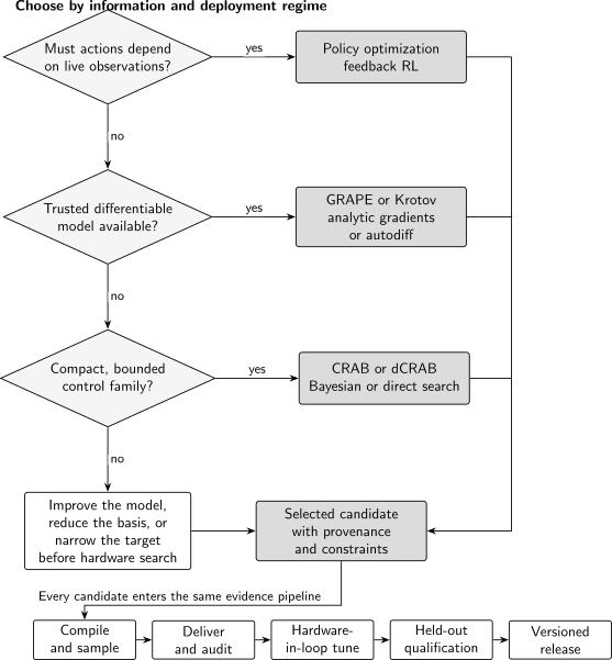
A method-selection map based on the deployed control object, model access, parameter dimension, and experimental cost. The lower pipeline is mandatory for every branch: an optimized representation must still be compiled, delivered, refined when necessary, independently qualified, and released as a versioned artifact.

Representations Determine the Search

Suppose a duration $T$ is divided into $N$ samples for each of $m$ control channels. An unrestricted sampled representation contains roughly $mN$ variables. That may be natural for an adjoint method in simulation and hopeless for a noisy hardware-only search. A compact basis with $K$ terms may reduce the dimension to order $mK$, but at the cost of excluding waveform features outside that basis.

The representation should be chosen jointly with the delivery chain:

• piecewise-constant samples match many propagators but can introduce sharp spectral components;
• spline knots give smooth interpolation but must be sampled deterministically;
• Fourier coefficients express bandwidth limits but handle localized features inefficiently;
• analytic pulse families are interpretable and compact but encode strong prior assumptions;
• controller-native primitives reduce compilation ambiguity but may limit the search space;
• conditional policies require a finite observation alphabet, state memory, and bounded branch latency.

Increasing dimension does not monotonically improve deployed performance. It can increase expressivity while worsening conditioning, sample complexity, overfitting, compilation sensitivity, and reproducibility. Report performance as a function of dimension and budget, not only the best result found.

Robustness Is a Distributional Claim

A robust pulse is robust to a declared set or distribution of perturbations, not to uncertainty in general. Let $L(\boldsymbol\alpha,\theta)$ be a physical loss under uncertain parameters $\theta$. Three common risk summaries are

$$\begin{aligned} J_{\mathrm{mean}} &= \mathbb E_{\theta}[L], \\ J_{\mathrm{worst}} &= \sup_{\theta\in\Theta} L, \\ J_{\mathrm{tail}} &= \operatorname{CVaR}_{q}(L). \end{aligned}$$

Mean loss can hide rare failures. Worst-case loss may be dominated by an implausible corner or be difficult to optimize. Conditional value at risk summarizes the upper-loss tail at a declared quantile $q$. None is meaningful without the uncertainty set, sampling rule, correlations, and physical units.

Training and validation uncertainty samples must be separated. For example, optimize on a coarse ensemble of detuning and amplitude offsets, then validate on new points, correlated perturbations, updated transfer-function models, and measured drift trajectories. A dense plot on the same grid used by the optimizer is a visualization of training performance, not an out-of-sample robustness test.

Robustness also has time semantics. A candidate can tolerate static detuning within one circuit yet fail under drift across an hour, or tolerate slow drift yet fail under fast noise within a gate. The uncertainty model must identify which parameters are constant per pulse, per shot, per batch, or dynamically varying within the evolution.

From Optimizer Output to Delivered Control

The physical system does not receive the optimizer’s abstract vector. A common delivery map is

$$\boldsymbol\alpha \xrightarrow{\ P\ } u_{\mathrm{analytic}}(t) \xrightarrow{\ S\ } u[n] \xrightarrow{\ Q\ } \widetilde u[n] \xrightarrow{\ G\ } u_{\mathrm{delivered}}(t),$$

where $P$ evaluates the pulse parametrization, $S$ samples it, $Q$ applies quantization and clipping, and $G$ is the delivery transfer chain. Frequency mixing, frame updates, channel alignment, filters, predistortion, trigger latency, and crosstalk may all enter this map.

There are three defensible strategies:

• include differentiable approximations to the delivery map in model-based optimization;
• optimize directly in a controller-native representation;
• treat the residual mismatch as a small hardware-in-the-loop correction problem.

Whatever strategy is chosen, qualification must run the exact serialized artifact that would be released. Reconstructing a “nearly equivalent” pulse from plotting data is not a valid test. The Pulse-Level Control contract specifies the sample grid, units, frames, channel map, transformations, and certificate needed for executable equivalence.

Evidence Ladder

Optimization and qualification should use an explicit evidence ladder. Each rung answers a different question.

Evidence	Question answered	What it does not establish
training objective	did the optimizer improve its own score?	physical fidelity or generalization
independent simulation	does the candidate survive a changed solver, grid, or model?	hardware performance
pulse audit	is the serialized artifact legal and faithfully delivered?	target operation quality
calibration metric	does a targeted hardware experiment improve?	complete gate or channel quality
independent characterization	does a held-out protocol confirm the operation?	workload-level benefit
workload or logical metric	does the change help the intended computation?	transfer to other contexts or epochs

A useful diagnostic is the simulation-to-experiment gap

$$\Delta_{\mathrm{sim\to exp}} = L_{\mathrm{exp}}(\boldsymbol\alpha^*) - L_{\mathrm{sim}}(\boldsymbol\alpha^*).$$

The sign and magnitude depend on metric conventions, finite-shot uncertainty, and context. A large gap is evidence about the entire modeling and delivery pipeline; it is not automatically evidence that the numerical optimizer failed.

Training and qualification metrics should differ enough to resist proxy gaming. For example, tune a gate with an interleaved randomized-benchmarking signal, then qualify leakage, phase, crosstalk, and a separately seeded benchmark. When randomized benchmarking is used, its assumptions and fitted estimand must be stated as described in Metrics for Quantum Hardware; they are not defined by the optimizer.

Experimental Budget and Nonstationarity

For hardware search, the relevant resource is often total device occupation, not the number of parameter updates. A rough shot count is

$$B_{\mathrm{shots}} = N_{\mathrm{candidates}} N_{\mathrm{settings}} N_{\mathrm{shots/setting}}.$$

Wall-clock cost also includes compilation, queueing, reset, waveform upload, latency, recalibration, and analysis. Parallel evaluation may reduce elapsed time while increasing crosstalk or changing thermal conditions. Every method comparison should declare both query counts and physical resource accounting.

The objective may drift during optimization. If $J_t(\boldsymbol\alpha)$ changes appreciably over the search, a score difference between candidates tested at distant times confounds pulse quality with device state. Useful countermeasures include randomized evaluation order, repeated incumbent sentinels, interleaved references, contextual covariates, shorter batches, and change-point alarms. If a regime change is detected, the run should be split or aborted rather than fitted as if all samples came from one stationary objective.

Hardware exploration must be bounded. Candidate generation should enforce static constraints before upload; the controller should enforce runtime limits; monitoring should define abort conditions; and the calibration service should have a recoverable incumbent. Reinforcement learning does not justify unsafe exploration, and “the agent chose it” is not an acceptable provenance record.

Worked Method Choices

Smooth single-qubit pulse with a reliable model

Suppose a calibrated Hamiltonian and transfer function predict a weakly anharmonic qubit accurately over the pulse duration. The task is a short gate with bounded amplitude, derivative, and leakage. A differentiable compact parametrization or filtered GRAPE is a strong baseline. Optimize across a small detuning and amplitude ensemble, verify gradients, refine the simulation grid, and compare against the incumbent analytic pulse.

The model-based result should then be serialized through the real pulse stack and tested on hardware. If the remaining discrepancy is smooth and low-dimensional, expose a few amplitude, quadrature, detuning, or basis coefficients to a bounded local hardware search. There is little reason to begin with a high-capacity reinforcement-learning policy when no sequential observation is available and a good gradient already exists.

Entangling gate with uncertain parasitic couplings

For an entangling gate, a nominal model may capture the desired interaction but miss crosstalk, spectator shifts, and delivery distortion. Use the model to find a feasible seed and to eliminate obviously poor regions. Then perform hardware refinement in a small basis using a black-box method whose evaluation budget matches device access.

The training score must be sensitive to the desired nonlocal operation, while qualification separately checks local phases, leakage, spectators, and drift. The final artifact is accepted only relative to a specified qubit neighborhood and calibration epoch. A pulse optimized on one pair is not automatically portable to another pair with the same nominal topology.

Conditional reset from a noisy measurement record

If each action depends on a stream of imperfect observations, the output is a policy rather than one fixed pulse. A recurrent or belief-state policy may be useful when the physical state is partially observed. Model-based policy optimization can exploit a differentiable stochastic simulator; model-free reinforcement learning may be considered when direct interaction and a well-defined safe action set are available.

Now latency, observation preprocessing, memory state, branch timing, and fallback actions become part of the artifact. Evaluation must include rare records, detector drift, delayed observations, controller saturation, and the cost of extra measurements. The stochastic theory and causal distinctions are developed in Measurement-Based Feedback.

Reproducible Optimization Records

A mature optimization run should produce an immutable record containing:

• target operation, basis ordering, rotating frame, and phase conventions;
• model equations, parameter values, uncertainty samples, and model version;
• pulse or policy representation, bounds, filters, and controller target;
• objective terms, units, weights, estimators, and sign convention;
• optimizer implementation and version, hyperparameters, stopping rules, and random seeds;
• initial candidates, restarts, rejected runs, and baseline controls;
• compute backend, numerical tolerances, time grid, and gradient checks;
• device identifier, calibration snapshot, timestamps, contexts, and raw-data references for hardware evaluations;
• total simulations, circuits, shots, wall-clock time, and device occupation;
• training curves with uncertainty and incumbent evaluations;
• independent validation results, acceptance decision, approver, and rollback target;
• hashes of the source representation and final serialized artifact.

Reporting only the best fidelity and pulse image conceals selection bias. If $R$ random restarts were tried, the distribution across all $R$ attempts is part of the result. If hyperparameters were chosen using the claimed test set, that set became validation data and a new held-out test is needed.

Common Mistakes

• Choosing an algorithm before specifying the control representation and evaluation budget.
• Calling hardware-in-the-loop pulse tuning “real-time feedback” when the deployed pulse does not depend on observations within a run.
• Treating automatic differentiation as evidence that the simulator is physically accurate.
• Comparing optimizers by iteration count rather than simulations, circuits, shots, device occupation, and wall-clock time.
• Optimizing an illegal waveform and checking amplitude or bandwidth only after clipping and sampling.
• Reporting a state-transfer reward as gate fidelity.
• Using the same noise ensemble, random seeds, or device batches for training and robustness validation.
• Omitting the incumbent analytic pulse or a simpler optimizer from the baseline comparison.
• Selecting the best of many restarts and reporting only that run.
• Allowing a learned policy to explore actions outside hard safety and controller constraints.
• Releasing an optimizer output without versioned pulse metadata, qualification, and rollback.
• Interpreting one successful device epoch as evidence of portability or long-term robustness.

Exercises

1. Distinguish two loops

An optimizer proposes a fixed pulse, runs it on hardware, observes a terminal score, and updates the pulse for the next batch. Is the deployed pulse a measurement-feedback policy?

Solution

No. The optimization procedure forms a hardware-in-the-loop calibration loop, but each deployed pulse is fixed within an experimental trajectory. A measurement-feedback policy would choose an action during the trajectory from a contemporaneous observation or observation history. The two workflows have different latency, causal, and safety contracts.

2. Count the query budget

A black-box optimizer tests $36$ candidates. Each score averages $8$ circuit settings with $2{,}000$ shots per setting. Ten percent of batches are repeated as incumbent sentinels. Ignoring integer rounding, how many shots are used?

Solution

The candidate evaluations use

$$36\times 8\times 2{,}000 = 576{,}000$$

shots. A ten-percent sentinel overhead multiplies this by $1.10$, giving $633{,}600$ shots. A complete wall-clock budget would also include reset, upload, compilation, queueing, and analysis time.

3. Select a method family

You have a differentiable simulator, $1{,}200$ waveform variables, and enough compute for repeated propagation. Hardware access is limited to fifty final candidate evaluations. Which family is the natural first baseline, and how should the hardware budget be used?

Solution

An adjoint-gradient method such as GRAPE is the natural first baseline because it can obtain derivatives for many waveform variables without one full simulation per variable. Use simulation for the high-dimensional search, including constraints and uncertainty. Spend the scarce hardware budget on independent qualification and, if needed, a low-dimensional bounded refinement around the simulated candidate. A hardware-only search over all $1{,}200$ variables would be poorly matched to the query budget.

4. Diagnose a clipped optimum

An optimizer returns a waveform with peaks above the hardware limit. Engineers clip it before upload, and the measured score is poor. Why is increasing the amplitude penalty after the run not a sufficient validation argument?

Solution

The clipped waveform is a different control from the waveform whose simulated objective was optimized. A finite penalty does not prove feasibility, and postprocessing can change amplitude, phase, spectrum, and dynamics. The search should enforce the limit or include the exact clipping map in every objective evaluation, then reoptimize and qualify the serialized result.

5. Train and test robustness

A pulse is optimized on detuning offsets $\{-2,-1,0,1,2\}\,\mathrm{MHz}$. Propose a minimal held-out robustness test.

Solution

Test new offsets between and beyond the training values, for example $\{-2.5,-1.5,-0.5,0.5,1.5,2.5\}\,\mathrm{MHz}$, without further pulse tuning. Also vary at least one coupled uncertainty such as amplitude scale or transfer- function parameters, because a one-dimensional sweep cannot support a broad robustness claim. Report uncertainty from finite shots and identify which points are inside versus outside the declared operating region.

6. Reward is not the target

An agent receives reward equal to the measured population in $\lvert1\rangle$ after starting in $\lvert0\rangle$. It reaches reward $0.999$. Give two reasons this does not establish a high-fidelity $X_\pi$ gate.

Solution

First, one state-transfer experiment does not determine a gate: the operation may give incorrect phases or act incorrectly on $\lvert1\rangle$ and superpositions. Second, the measured population includes state-preparation and measurement effects and may be insensitive to leakage or incoherent transfer. Independent process-sensitive and leakage-sensitive qualification is needed.

7. Detect nonstationarity

During a four-hour optimization, the incumbent score measured every twentieth candidate degrades steadily. How should candidate comparisons and the final claim change?

Solution

Raw scores from widely separated times should not be treated as samples of one stationary objective. Use the interleaved incumbent to model or bound temporal drift, compare candidates in nearby blocks, and test for a regime change. If the operating regime changed, stop or segment the run and requalify the final candidate against a current incumbent. The report should include the drift and must not attribute the entire score change to optimization.

8. Release decision

A new pulse improves its training score by $3\%$ and an independent gate metric by $0.4\%$, but increases leakage beyond the published operating limit. Should the calibration service release it?

Solution

No. The leakage limit is a hard acceptance condition, so improvements in other metrics do not make the candidate releasable. The service should reject or quarantine the candidate, retain the valid incumbent, record the evidence, and return the leakage failure to the optimization stage as a constraint or target revision.

Research Status

Gradient-based quantum optimal control, reduced-basis search, robust ensemble objectives, and device-level closed-loop refinement are established methods. Their relative performance remains strongly dependent on the model, pulse representation, target, constraints, noise, and cost accounting. Claims that one optimizer is generally superior are not supported by success on a single system or by comparisons with unequal evaluation budgets.

Reinforcement learning has produced important numerical and experimental demonstrations, including model-free state preparation, feedback policies, and gate-set design. It is an active research area rather than a universal replacement for optimal-control solvers. Open problems include sample-efficient hardware learning, safe exploration, transfer across devices and epochs, uncertainty-calibrated policies, reliable sim-to-real adaptation, rare-event validation, and comparisons against strong non-learning baselines.

At larger scale, control optimization also interacts with crosstalk, simultaneous operations, scheduling, calibration drift, and workload context. The optimization unit may need to grow from one isolated gate to a local spatiotemporal region, but increasing scope rapidly increases model and validation burden. Scalable deployment therefore depends as much on typed interfaces, provenance, resource accounting, and conservative release policy as on optimizer sophistication.

Further Connections

• Optimal Control is the canonical home for dynamical objectives, constraints, adjoint gradients, GRAPE, Krotov methods, and robustness ensembles.
• Variational Quantum Algorithms owns the gate-level hybrid objective, parameter-shift, quantum-geometry, trainability, and algorithm-validation framework that overlaps with control optimization.
• Pulse-Level Control defines how optimized controls are sampled, transformed, serialized, and certified for a controller target.
• Calibration Loops owns device access, dependency graphs, drift monitoring, candidate acceptance, publication, and rollback.
• Control, Readout, and Calibration develops the physical delivery chain and representative experiments used to estimate control parameters.
• Measurement-Based Feedback develops causal feedback from quantum measurement records.
• Metrics for Quantum Hardware distinguishes physical, gate, readout, logical, and workload estimands used in qualification.
• Error-Aware Compilation consumes qualified gate alternatives and dated calibration evidence when choosing mappings and schedules.
• Optimal Control Toy Problems provides small reproducible numerical contracts for checking control implementations.

References

1. C. Brif, R. Chakrabarti, and H. Rabitz, “Control of quantum phenomena: past, present and future,” New Journal of Physics 12, 075008 (2010), doi:10.1088/1367-2630/12/7/075008.
2. N. Khaneja, T. Reiss, C. Kehlet, T. Schulte-Herbrüggen, and S. J. Glaser, “Optimal control of coupled spin dynamics: design of NMR pulse sequences by gradient ascent algorithms,” Journal of Magnetic Resonance 172, 296–305 (2005), doi:10.1016/j.jmr.2004.11.004.
3. S. J. Glaser et al., “Training Schrödinger’s cat: quantum optimal control,” European Physical Journal D 69, 279 (2015), doi:10.1140/epjd/e2015-60464-1.
4. T. Caneva, T. Calarco, and S. Montangero, “Chopped random-basis quantum optimization,” Physical Review A 84, 022326 (2011), doi:10.1103/PhysRevA.84.022326.
5. N. Rach, M. M. Müller, T. Calarco, and S. Montangero, “Dressing the chopped-random-basis optimization: a bandwidth-limited access to the trap-free landscape,” Physical Review A 92, 062343 (2015), doi:10.1103/PhysRevA.92.062343.
6. D. J. Egger and F. K. Wilhelm, “Adaptive hybrid optimal quantum control for imprecisely characterized systems,” Physical Review Letters 112, 240503 (2014), doi:10.1103/PhysRevLett.112.240503.
7. M. H. Goerz et al., “Krotov: a Python implementation of Krotov’s method for quantum optimal control,” SciPost Physics 7, 080 (2019), doi:10.21468/SciPostPhys.7.6.080.
8. H. Ball et al., “Software tools for quantum control: improving quantum computer performance through noise and error suppression,” Quantum Science and Technology 6, 044011 (2021), doi:10.1088/2058-9565/abdca6.
9. M. Bukov et al., “Reinforcement learning in different phases of quantum control,” Physical Review X 8, 031086 (2018), doi:10.1103/PhysRevX.8.031086.
10. M. Y. Niu, S. Boixo, V. N. Smelyanskiy, and H. Neven, “Universal quantum control through deep reinforcement learning,” npj Quantum Information 5, 33 (2019), doi:10.1038/s41534-019-0141-3.
11. Y. Baum et al., “Experimental deep reinforcement learning for error-robust gate-set design on a superconducting quantum computer,” PRX Quantum 2, 040324 (2021), doi:10.1103/PRXQuantum.2.040324.
12. V. V. Sivak, A. Eickbusch, H. Liu, B. Royer, I. Tsioutsios, and M. H. Devoret, “Model-free quantum control with reinforcement learning,” Physical Review X 12, 011059 (2022), doi:10.1103/PhysRevX.12.011059.
13. J. Kelly et al., “Optimal quantum control using randomized benchmarking,” Physical Review Letters 112, 240504 (2014), doi:10.1103/PhysRevLett.112.240504.
14. C. P. Koch et al., “Quantum optimal control in quantum technologies: strategic report on current status, visions and goals for research in Europe,” EPJ Quantum Technology 9, 19 (2022), doi:10.1140/epjqt/s40507-022-00138-x.