Error-Aware Compilation

Short Definition

Error-aware compilation chooses among semantically acceptable, target-legal implementations using evidence about the present device: operation quality, duration, relaxation and dephasing, leakage, readout, crosstalk, disabled resources, drift, and uncertainty. Its job is not to make an imperfect processor noiseless. Its job is to spend the available hardware quality where a particular computation benefits from it most.

A useful abstract contract is

$$\begin{aligned} &\mathsf{EACompile} \bigl( C,\Theta,\mathcal D,t_{\mathrm{exec}},\mathcal O,\mathcal B \bigr) \\ &\qquad \longrightarrow \bigl(C^\star,\mathcal K\bigr). \end{aligned}$$

Here $C$ is the program, $\Theta$ is a versioned target contract, $\mathcal D$ is dated device evidence, $t_{\mathrm{exec}}$ is the anticipated execution time, $\mathcal O$ states the operational objective, and $\mathcal B$ bounds compilation and characterization resources. The output $C^\star$ is a selected executable and $\mathcal K$ is a decision certificate.

This page is the canonical home for turning device evidence into compiler features, defining risk-aware cost functions, ranking legal candidates, handling stale or uncertain calibration data, and validating the selection. Qubit Mapping and Routing owns connectivity legalization and map evolution. Control, Readout, and Calibration owns how device parameters are estimated and maintained. Noise in Quantum Information owns the physical and channel taxonomy. Error mitigation and fault tolerance change the execution or encoding contract; they are not synonyms for choosing a lower-risk compilation.

The Decision Contract

Let $\mathcal X(C,\Theta)$ be the set of implementations that satisfy the declared semantics and target legality:

$$\begin{aligned} \mathcal X(C,\Theta) = \bigl\{ x: &\ \mathsf{Semantics}(x) \simeq \\ &\ \mathsf{Semantics}(C), \\ &\ \mathsf{Legal}(x,\Theta)=1 \bigr\}. \end{aligned}$$

The equivalence relation $\simeq$ may allow global phase, an approximation tolerance, ancillas returned in a specified state, a final qubit permutation, or classical relabeling. Those permissions must already be explicit. Noise awareness does not license a compiler to silently change the algorithm.

In practice the compiler searches only a bounded candidate subset $\mathcal X_{\mathcal B}\subseteq\mathcal X$. It selects

$$x^\star \in \operatorname*{arg\,min}_{x\in\mathcal X_{\mathcal B}} \widehat L \bigl( x;\mathcal D,t_{\mathrm{exec}},\mathcal O \bigr),$$

where $\widehat L$ is a predicted loss, not an observed theorem about the future run. The distinction matters: the candidate generator, score model, calibration sample, and queue delay can all change the winner.

Contract component	Minimum content	Why it matters
program semantics	outputs, observables, approximation and phase conventions	defines which candidates are equivalent
target	native operations, topology, durations, concurrency and resource limits	defines legality
evidence	estimate, uncertainty, context, timestamp, method and calibration identifier	defines what the score actually knows
execution horizon	expected dispatch time and permitted freshness window	exposes staleness
objective	task metric, surrogate, weights and risk attitude	defines what “better” means
search budget	timeout, candidate count, solver gap and random seed	bounds the claim
output	executable, final maps, schedule and evidence certificate	makes the decision reproducible

An error-aware compiler is therefore a decision system with provenance, not a switch labeled “optimize fidelity.”

From Device Evidence to Compiler Features

A compiler should not ingest a bare scalar called an error rate. A useful feature record for quantity $j$ is

$$d_j = \bigl( \widehat\eta_j,\, u_j,\, t_j,\, \kappa_j,\, \nu_j \bigr),$$

where $\widehat\eta_j$ is the estimate, $u_j$ describes uncertainty, $t_j$ is the acquisition time, $\kappa_j$ records context, and $\nu_j$ identifies the estimation method and version. Context can include the gate parameters, neighbor activity, direction, preparation and measurement settings, pulse family, and processor mode.

The delay between evidence and use is

$$\Delta t_j = t_{\mathrm{exec}}-t_j.$$

Freshness is not determined by $\Delta t_j$ alone. A stable quantity measured hours ago may be more useful than a volatile quantity measured minutes ago. A compiler policy may attach a decay weight such as

$$w_j(t_{\mathrm{exec}}) = \exp\left( -\frac{\Delta t_j}{\tau_j^{\mathrm{valid}}} \right),$$

but $\tau_j^{\mathrm{valid}}$ is a model of evidence relevance, not the qubit’s $T_1$ or $T_2$.

Evidence supplied	Plausible compiler use	Important failure mode
one- and two-qubit benchmark rates	rank gate families, sites and edges	a benchmark decay is not a Bernoulli failure probability
operation durations	schedule exposure and critical paths	duration alone omits driven and idle noise
$T_1$, $T_2$, or Ramsey data	estimate state-dependent idle risk	one timestamp may miss drift and non-Markovianity
leakage and seepage estimates	avoid high-leakage operations or long live ranges	leakage is not captured by a qubit-only Pauli model
asymmetric readout confusion	place important measured outputs	the expected bit distribution may be unknown
simultaneous-operation tests	impose conflicts or crosstalk penalties	pair tests may miss three-body and mode dependence
disabled components	forbid candidates	a stale availability map can make output illegal
historical time series	estimate volatility and robust ranges	yesterday’s distribution need not describe today

The Circuit Intermediate Representations page explains why these data need types, units, scope, and provenance. The Metrics for Quantum Hardware page owns the definitions of the underlying hardware metrics.

Independent-Error Scores

A common first surrogate multiplies reported operation successes:

$$\widehat P_{\mathrm{ind}}(x) = \prod_{g\in x} \bigl(1-\widehat r_g\bigr) \prod_{m\in x} \bigl(1-\widehat r_m\bigr).$$

Taking a negative logarithm converts the product into an additive path cost:

$$\begin{aligned} J_{\mathrm{ind}}(x) &= -\log\widehat P_{\mathrm{ind}}(x) \\ &= \sum_{g\in x} -\log\bigl(1-\widehat r_g\bigr) \\ &\quad+ \sum_{m\in x} -\log\bigl(1-\widehat r_m\bigr). \end{aligned}$$

For small $\widehat r$,

$$-\log(1-\widehat r) = \widehat r + O(\widehat r^2),$$

so minimizing the log score resembles minimizing a weighted error count. This is useful for shortest paths, assignment, integer programming, and fast candidate ranking.

It is still only a surrogate. The product assumes independent, context-invariant events. A randomized-benchmarking decay parameter is not literally the probability that one occurrence of a named gate fails. Coherent overrotations may add or cancel. Leakage survives beyond one gate. Readout errors depend on the prepared state. Crosstalk depends on the schedule. Temporally correlated noise violates the factorization itself.

Call $\widehat P_{\mathrm{ind}}$ a calibration-derived product score unless its probabilistic interpretation has been independently justified. Do not rename it “circuit fidelity” merely because its value lies between zero and one.

Multi-Component Objectives

A broader loss can separate terms:

$$\begin{aligned} \widehat L(x) =\;& \alpha J_{\mathrm{gate}}(x) + \beta J_{\mathrm{idle}}(x) \\ &+ \gamma J_{\mathrm{read}}(x) + \delta J_{\mathrm{xtalk}}(x) \\ &+ \epsilon J_{\mathrm{leak}}(x) + \zeta J_{\mathrm{resource}}(x). \end{aligned}$$

The coefficients are not universal constants. They encode a decision policy and must be reported. A circuit returning a full bit string may care strongly about readout assignment. An expectation-estimation workload may tolerate some outcomes differently. A dynamic circuit can be dominated by measurement, reset, and classical-feedback latency. A fault-tolerant subroutine should ultimately be judged by logical failure and resource cost, not a product of physical gate benchmarks.

Whenever possible, predict the operational loss directly. Examples include:

• probability of a declared correct output for a checkable circuit;
• total-variation or Hellinger distance between output distributions;
• bias, variance, or mean-squared error of a target observable;
• logical failure probability per round or operation;
• accepted samples per unit wall time;
• an application utility with explicit classical postprocessing.

When direct prediction is infeasible, report which surrogate is used and validate whether it preserves the candidate ranking relevant to the workload. A model can be badly calibrated in absolute value yet useful for ranking; it can also predict plausible values while ranking candidates incorrectly.

Pareto decisions

Compressing everything into one scalar can hide meaningful tradeoffs. Define a cost vector

$$\mathbf J(x) = \bigl( J_{\mathrm{error}}, T_{\mathrm{exec}}, T_{\mathrm{compile}}, N_{\mathrm{cal}}, N_{\mathrm{shots}} \bigr).$$

A candidate $x$ dominates $y$ if every component is no worse and at least one is better. Nondominated candidates form a Pareto set. A scheduler can then choose according to a declared latency or calibration budget instead of smuggling that preference into undocumented weights.

Uncertainty and Rank Stability

Finite characterization shots, fit uncertainty, drift, context mismatch, and queue delay make $\eta$ uncertain. Three defensible objectives are:

$$\begin{aligned} J_{\mathrm{mean}}(x) &= \mathbb E_{\eta\mid\mathcal D} \bigl[ L(x,\eta) \bigr], \\ J_{\mathrm{rob}}(x) &= \max_{\eta\in\mathcal U(\mathcal D)} L(x,\eta), \\ J_{\mathrm{risk}}(x) &= \mathbb E[L(x,\eta)] \\ &\quad+ \lambda\, \operatorname{CVaR}_{\alpha} \bigl( L(x,\eta) \bigr). \end{aligned}$$

The conditional value at risk can be written

$$\begin{aligned} \operatorname{CVaR}_{\alpha}(L) &= \min_z \Biggl[ z + \frac{1}{1-\alpha} \\ &\qquad{}\times \mathbb E \bigl[ (L-z)_+ \bigr] \Biggr]. \end{aligned}$$

Mean optimization is appropriate only when the evidence distribution and loss are credible. Worst-case optimization protects against a declared uncertainty set but may be overly conservative. A tail-risk objective interpolates between them.

The compiler should also estimate rank stability. For two candidates,

$$\Delta L(\eta) = L(x_2,\eta)-L(x_1,\eta).$$

If the uncertainty interval for $\Delta L$ crosses zero, the data do not support a stable ordering. The right action may be to choose the simpler candidate, run a targeted characterization, compile a small portfolio, or report a tie. Extra decimal places do not resolve epistemic uncertainty.

Historical calibration can help when immediate data are unavailable, but it should be conditioned on relevant modes and monitored for distribution shift. The acquisition cost also belongs in the decision: a fresh characterization that consumes the entire execution window can be worse than a robust choice from older data.

Error-Aware Placement and Routing

Connectivity defines which routes are legal. Error awareness ranks those routes. On a fixed coupling graph, assign edge weights

$$w_e = -\log \bigl( 1-\widehat r_e \bigr),$$

and site or readout weights analogously. A minimum-hop path and a minimum-weight path need not agree. Nor must the lowest-weight path minimize scheduled loss, because its gates may serialize or overlap with hostile neighbors.

Consider two legal implementations of a measured output. Candidate $A$ uses three two-qubit operations with reported rate $0.006$ and a readout with rate $0.025$. Candidate $B$ uses two two-qubit operations at $0.014$ and a readout at $0.008$. Their independent scores are

$$\begin{aligned} \widehat P_A &= (0.994)^3(0.975) \simeq 0.9576, \\ \widehat P_B &= (0.986)^2(0.992) \simeq 0.9644. \end{aligned}$$

The proxy selects $B$: its gates look worse individually, but it uses fewer of them and ends on a better readout site. This is a ranking under a model, not proof that $B$ will have higher experimental fidelity.

Error-aware routing can influence:

• the initial placement of high-degree or long-lived program qubits;
• which physical edge carries repeated entangling operations;
• which of several shortest SWAP paths is used;
• whether a final permutation is accepted rather than restored;
• where measured outputs finish;
• whether an isomorphic embedding is substituted after routing;
• when a marginally longer route avoids a volatile or disabled component.

The route certificate remains the authority for map evolution and legality. The error-aware certificate adds the dated evidence and ranking model.

Crosstalk-Aware Scheduling

Let $y_{gh}=1$ when operations $g$ and $h$ overlap in a context declared relevant. A pairwise scheduling penalty is

$$J_{\mathrm{xtalk}} = \sum_{g\lt h} \xi_{gh}y_{gh},$$

where $\xi_{gh}$ may be inferred from simultaneous benchmarking or another contextual experiment. Pairwise additivity is an approximation; triple interactions and global modes can invalidate it.

Serializing every gate eliminates concurrency but increases live time. A simple comparison illustrates the tradeoff. Suppose parallel execution incurs a success factor $1-\chi$, while serialization adds delay $\Delta$ to a coherence-sensitive state with approximate factor $e^{-\Delta/T_2}$. Serialization is favored by this model when

$$\begin{aligned} e^{-\Delta/T_2} &\gt 1-\chi, \\ \Delta &\lt -T_2\log(1-\chi). \end{aligned}$$

For $T_2=80\,\mu\mathrm{s}$ and $\chi=0.06$, the threshold is about $4.95\,\mu\mathrm{s}$. A $3\,\mu\mathrm{s}$ delay favors serialization in this model; an $8\,\mu\mathrm{s}$ delay favors overlap. Real dephasing, driven-gate error, spectator state, leakage, and echo structure can change the answer, so the inequality is a decision aid rather than a device law.

The scheduler needs operation intervals, exclusion resources, conditional rates, state live ranges, measurement deadlines, and classical latencies. This is why error-aware compilation cannot be reduced to assigning static weights to a coupling graph.

Gate Family and Synthesis Choices

Two implementations can be exactly equivalent yet expose different physical error channels. The compiler may choose:

• one native entangler family over another;
• an interaction direction or locally equivalent orientation;
• a continuously parameterized entangler instead of repeated maximal gates;
• a mirrored or sign-reversed decomposition with lower total interaction angle;
• a decomposition that trades entangling operations for local rotations;
• an approximate synthesis with a declared algorithmic tolerance;
• a frame update instead of a driven physical operation.

Continuously parameterized gates make the boundary especially clear. The gate decomposer establishes which exact or approximate words implement the target. The error-aware selector ranks those words using angle-, pair-, and context-dependent evidence. The pulse-control layer realizes the selected native operation.

Algorithmic approximation error and physical implementation error must not be added unless they use compatible metrics. For channels $\mathcal U$, $\mathcal V$, and a physical implementation $\widetilde{\mathcal V}$, the diamond norm gives the rigorous triangle bound

$$\begin{aligned} \frac12 \left\| \widetilde{\mathcal V}-\mathcal U \right\|_{\diamond} \leq\;& \frac12 \left\| \widetilde{\mathcal V}-\mathcal V \right\|_{\diamond} \\ &+ \frac12 \left\| \mathcal V-\mathcal U \right\|_{\diamond}. \end{aligned}$$

A calibration-derived product score is not a diamond-norm estimate, so it cannot simply be inserted into this bound.

Readout-Aware Decisions

Readout is generally asymmetric. Define

$$\begin{aligned} e_{1\mid0} &= \Pr(\widetilde m=1\mid m=0), \\ e_{0\mid1} &= \Pr(\widetilde m=0\mid m=1). \end{aligned}$$

With observed outcomes as rows and ideal outcomes as columns, the one-qubit confusion matrix is

$$M = \begin{pmatrix} 1-e_{1\mid0} & e_{0\mid1} \\ e_{1\mid0} & 1-e_{0\mid1} \end{pmatrix}.$$

If a trustworthy task model predicts probabilities $p_0$ and $p_1$, the expected bit-error proxy is

$$\widehat r_{\mathrm{read}} = p_0e_{1\mid0} + p_1e_{0\mid1}.$$

Using $(e_{1\mid0}+e_{0\mid1})/2$ instead assumes balanced ideal outcomes. That may be appropriate for a benchmark and wrong for a workload. For an unknown quantum output, using a guessed distribution can introduce a hidden task prior into placement.

Readout-aware compilation maps important measured values to suitable channels, preserves the final physical-to-program permutation, and respects simultaneous-readout conflicts. Measurement-error mitigation instead estimates or corrects noisy output statistics; it is a separate contract.

A Time-Dependent Compilation Loop

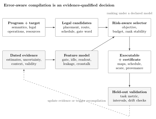
Error-aware compilation ranks only semantically valid, target-legal candidates. Dated evidence and uncertainty enter the score; held-out execution data test the ranking and can trigger later characterization or recompilation.

Three timing policies are common:

Policy	Advantage	Risk
static compilation	reusable artifact and low dispatch latency	evidence may not match the execution epoch
batch-aware compilation	amortizes characterization across a campaign	queue order and within-batch drift matter
just-in-time compilation	can use fresher targeted evidence	characterization and compile latency consume the freshness window

A useful validity condition is

$$t_{\mathrm{exec}} \in \mathcal I_{\mathcal D},$$

where $\mathcal I_{\mathcal D}$ is the declared evidence-validity interval. If execution slips outside it, the runtime should re-score, recompile, request new data, or explicitly accept the stale-evidence policy. Silent use of stale scores makes provenance misleading.

Compilation and calibration form a feedback loop but should not use the same data twice without accounting for selection. Characterization data may select a candidate; independent application or validation shots should assess the claim. Otherwise the compiler can overfit measurement noise in the calibration sample.

Search Methods

Method	Strength	Limitation
exact SMT, MILP, or constraint optimization	proves optimality within a declared model and candidate space	scales poorly and inherits model error
graph and local-search heuristics	fast placement, path, and schedule changes	local choices and pass order can miss better combinations
post-routing isomorphic embeddings	inexpensive remapping without rerouting	cannot repair a poor routed interaction pattern
candidate portfolios	exposes rank uncertainty and supports late binding	increases compile, storage, and validation cost
learned ranking	can model nonlinear context from data	vulnerable to distribution shift, leakage, and opaque failure
online bandit or adaptive selection	learns from current execution batches	exploration consumes shots and complicates independence

No selector can recover a candidate that its generator never produced. Comparing scoring functions while giving them different search spaces confounds the result. Exact optimality means optimal for the stated surrogate, constraints, evidence snapshot, and candidate set; it does not mean physically optimal under the unknown device process.

Learned models need especially careful splits. Training and test circuits should not share near-duplicate compiled structures across the split, and future calibration epochs should be evaluated as temporal holdouts. A model that memorizes which edge was best yesterday is not a general noise model.

Verification and Decision Certificates

An error-aware output requires several distinct checks:

1. Semantic verification: the selected circuit satisfies the equivalence and approximation contract.
2. Target verification: every operation, resource, timing relation, and final map is legal for the target version.
3. Score replay: an independent implementation recomputes the score from the recorded evidence.
4. Uncertainty audit: the claimed ordering survives the declared uncertainty analysis, or the certificate records an unresolved tie.
5. Empirical validation: held-out runs test the operational metric under the stated execution conditions.

The certificate $\mathcal K$ should record:

• source and executable hashes;
• IR, target, compiler, pass, and solver versions;
• semantic equivalence and approximation conventions;
• candidate-generation method and search budget;
• calibration identifiers, timestamps, units, contexts, estimates, and uncertainties;
• anticipated and actual execution times;
• objective terms, normalization, weights, and risk parameters;
• selected candidate, alternatives considered, score gap, and solver gap;
• initial and final qubit maps, schedule, and measurement decoding;
• random seeds and tie-breaking rules;
• validation circuits, shots, metrics, intervals, and raw-result identifiers.

A predicted score and a measured outcome answer different questions. The score explains the compiler’s decision under a model. The validation result supports a claim about executions sampled from a specified device epoch.

Benchmarking Error-Aware Compilers

A defensible comparison controls:

• input circuits, parameter bindings, observables, and output conventions;
• target topology, native alphabet, queue conditions, and calibration epoch;
• semantic tolerance and allowed final permutations;
• candidate-generation, compile-time, memory, and characterization budgets;
• optimization and decomposition before and after the tested pass;
• number of compiler seeds and execution shots;
• metric definition, uncertainty interval, and multiple-comparison policy;
• whether calibration, tuning, and validation data are disjoint;
• hardware time, classical compilation time, and discarded runs.

Report at least one structural metric, one predicted metric, and one held-out operational metric. Structural metrics include entangling count, depth, duration, and idle exposure. Predicted metrics include the declared calibration-derived loss. Operational metrics depend on the task: correct answer probability, distribution distance, observable error, or logical failure.

Evaluate across several calibration epochs. A same-day win on one processor shows that the method found a useful choice in that setting. It does not show that the objective is universally accurate or that the compiler dominates on other platforms. Include cases where error awareness makes no significant difference and cases where stale or misleading evidence hurts.

Common Mistakes

• Calling every hardware-aware legality pass error-aware.
• Treating an RB or vendor error number as a per-gate failure probability.
• Multiplying scalar rates while claiming to model coherent, correlated, or non-Markovian noise.
• Ignoring uncertainty, timestamp, queue delay, and calibration context.
• Minimizing two-qubit count while overlooking readout, idle, leakage, or crosstalk costs.
• Serializing all simultaneous operations to avoid crosstalk.
• Assuming the newest calibration point is necessarily the best predictor.
• Mixing approximation error with a physical proxy in incompatible metrics.
• Choosing measured-output qubits from a symmetric readout average when the confusion is asymmetric.
• Comparing selectors with different candidate spaces or compilation budgets.
• Evaluating on the same noisy sample used to choose the candidate.
• Reporting only the best compiler seed or best hardware epoch.
• Claiming physical optimality from optimality under a surrogate.
• Omitting the final qubit and classical-bit maps from the executable record.
• Conflating error-aware compilation with error mitigation or fault tolerance.

Exercises

1. Compute an independent product score

Candidate $A$ uses four two-qubit gates with reported rate $0.008$. Candidate $B$ uses three with rate $0.013$. Ignore all other errors. Which candidate does the independent product proxy prefer?

Solution

The two scores are

$$\begin{aligned} \widehat P_A &= (1-0.008)^4 \simeq 0.9684, \\ \widehat P_B &= (1-0.013)^3 \simeq 0.9615. \end{aligned}$$

The proxy prefers $A$ even though it uses one more gate. Equivalently, $-4\log(0.992)\lt-3\log(0.987)$. This does not establish that $A$ has higher experimental fidelity; it is the ranking under the independent scalar model.

2. Add readout to a route decision

Candidate $A$ has the two-qubit score from Exercise 1 and ends on a readout site with error $0.06$. Candidate $B$ ends on a site with error $0.01$. Re-rank the candidates using the product proxy.

Solution

Including readout gives

$$\begin{aligned} \widehat P_A' &= 0.9684(0.94) \simeq 0.9103, \\ \widehat P_B' &= 0.9615(0.99) \simeq 0.9519. \end{aligned}$$

The ranking reverses, so $B$ is preferred. The example shows why a route cannot be ranked solely by the edges used when its final map determines measurement channels.

3. Balance crosstalk and delay

Two gates incur a simultaneous-execution penalty $\chi=0.04$. Serializing them delays a coherence-sensitive state by $\Delta=2\,\mu\mathrm{s}$, with $T_2=70\,\mu\mathrm{s}$. Which schedule is favored by the simple threshold model?

Solution

The largest delay favoring serialization is

$$\begin{aligned} \Delta_{\max} &= -T_2\log(1-\chi) \\ &= -70\,\mu\mathrm{s}\log(0.96) \simeq 2.86\,\mu\mathrm{s}. \end{aligned}$$

Because $2\,\mu\mathrm{s}\lt2.86\,\mu\mathrm{s}$, the model favors serialization. The conclusion is conditional on its crude exponential dephasing and scalar crosstalk factors.

4. Detect a robust rank reversal

Two candidates have loss intervals

$$\begin{aligned} L_A&\in[0.020,0.055], \\ L_B&\in[0.030,0.040]. \end{aligned}$$

Their nominal losses are $0.025$ and $0.035$. Which candidate is selected by nominal and worst-case rules?

Solution

Nominal minimization selects $A$ because $0.025\lt0.035$. Worst-case minimization compares the upper endpoints and selects $B$ because $0.040\lt0.055$. The intervals overlap, so the evidence does not establish a uniform ordering. A certificate should record the risk rule rather than present either choice as unqualified.

5. Use asymmetric readout data

Site $A$ has $e_{1\mid0}=0.02$ and $e_{0\mid1}=0.10$. Site $B$ has $e_{1\mid0}=0.04$ and $e_{0\mid1}=0.03$. Rank the sites when the ideal output has $(p_0,p_1)=(0.9,0.1)$, then when it is balanced.

Solution

For the skewed output,

$$\begin{aligned} \widehat r_A &= 0.9(0.02)+0.1(0.10) = 0.028, \\ \widehat r_B &= 0.9(0.04)+0.1(0.03) = 0.039. \end{aligned}$$

Site $A$ is preferred. For balanced outputs,

$$\widehat r_A=0.060, \qquad \widehat r_B=0.035,$$

so $B$ is preferred. The workload prior changes the ranking; it must therefore be part of the objective contract.

6. Give a coherent-error counterexample

Explain why assigning the same positive scalar cost to every occurrence of $R_z(\theta)$ can mis-rank two implementations when the physical gate has a systematic overrotation.

Solution

Suppose the physical implementation is $\widetilde R_z(\theta)=R_z(\theta+\varepsilon)$ with nearly constant $\varepsilon$. Two identical rotations accumulate a coherent error $R_z(2\varepsilon)$. In contrast, an implementation using a rotation and a sign-reversed realization whose error also reverses can cancel the coherent offset.

A scalar positive cost added per occurrence predicts only accumulation. It does not encode the error generator, sign, frame, or surrounding gates, so it cannot represent cancellation. Randomization, context variation, or drift can change the example again.

7. Identify a Pareto set

Three candidates have

$$\begin{aligned} \mathbf J(A)&=(0.030,\,12,\,4),\\ \mathbf J(B)&=(0.025,\,15,\,6),\\ \mathbf J(C)&=(0.040,\,18,\,7), \end{aligned}$$

where components are predicted loss, execution time, and compile time, all to be minimized. Which candidates are Pareto optimal?

Solution

$A$ dominates $C$: it has lower predicted loss, execution time, and compile time. Neither $A$ nor $B$ dominates the other. $B$ has lower predicted loss, while $A$ has lower execution and compile times. The Pareto set is therefore $\{A,B\}$.

8. Audit staleness

A calibration snapshot was acquired at 09:00 with a declared validity window of two hours. Compilation finished at 09:20, but the queued job began at 11:35. What should the runtime record or do?

Solution

The execution lies outside the declared validity interval ending at 11:00. The runtime should not silently attach the old snapshot as current evidence. It should re-score or recompile with acceptable data, request targeted characterization, or execute under an explicit stale-evidence policy. The certificate should record acquisition, compilation, dispatch, and execution times and the action taken.

9. Design a fair hardware evaluation

Design an experiment to test whether an error-aware compiler improves a workload over a topology-only compiler.

Solution

Use the same source circuits, target, semantic tolerance, candidate-generation budget, optimization pipeline, compile timeout, final-map permissions, and execution allocation. Freeze or record all compiler versions and seeds. Acquire calibration data for selection, but reserve independent application shots for evaluation.

Run randomized or interleaved candidate order across several calibration epochs so drift does not favor one compiler. Report structural metrics, predicted scores, task-appropriate held-out metrics, confidence intervals, compiler time, characterization cost, queue delay, and failures. Include all prespecified circuits and seeds rather than only wins. This tests both average benefit and temporal robustness.

Research Status

Variability-aware placement, calibration-weighted mapping, crosstalk-aware scheduling, dated recompilation, and post-routing subgraph selection are established compiler strategies with experimental demonstrations. It is also well established that benchmarking numbers are context-dependent proxies and that processor behavior can drift.

There is no settled universal objective that predicts application performance across platforms, workloads, depths, and epochs. Active work includes richer contextual noise features, uncertainty-aware and online selection, continuously parameterized gate families, joint synthesis–routing–scheduling, learned rankers with distribution-shift controls, logical-level objectives, and cost-effective co-design of characterization and compilation. Claims should remain tied to the tested processor, candidate space, evidence epoch, budget, and operational metric.

Further Connections

• Qubit Mapping and Routing defines legal placement, movement, map evolution, scheduling constraints, and route certificates before error-aware ranking.
• Circuit Intermediate Representations carries target capabilities, calibration provenance, timing, uncertainty, and output-map metadata across passes.
• Gate Decomposition generates exact or approximate candidate words whose physical risks can then be compared.
• Circuit Optimization owns behavior-preserving simplification and translation validation independent of a dated noise ranking.
• Pulse-Level Control materializes a selected calibrated gate family as a typed, timed, frame-aware control program with a validation certificate.
• Calibration Loops produces the versioned estimates, uncertainty, validity intervals, context labels, and rollback state consumed by error-aware decisions.
• Optimal Control for Quantum Processors explains how new pulse or policy candidates are selected, refined under hardware budgets, and independently qualified before compilation may consume them.
• Quantum Software Stack places calibration acquisition, compilation, queueing, execution, and evidence in one operational lifecycle.
• Noise in Quantum Information distinguishes coherent, incoherent, leakage, crosstalk, SPAM, drift, and correlated mechanisms.
• Cycle Benchmarking validates a fixed scheduled layer in parallel context and makes timing, idles, spectators, Pauli dressing, and compiler provenance part of the estimand.
• Common Noise Models supplies explicit channels, parameter conventions, $T_1$–$T_2$ relations, leakage models, and model-checking cautions.
• Control, Readout, and Calibration owns estimands, calibration experiments, validation, feedback, and drift maintenance.
• Metrics for Quantum Hardware defines the hardware quantities that must not be conflated with application success.
• Quantum Channels and Noise develops the completely positive map language needed to reason beyond scalar error scores.

References

1. P. Murali, J. M. Baker, A. Javadi-Abhari, F. T. Chong, and M. Martonosi, “Noise-adaptive compiler mappings for noisy intermediate-scale quantum computers,” in Proceedings of ASPLOS 2019, 1015–1029 (2019), doi:10.1145/3297858.3304075.
2. S. S. Tannu and M. K. Qureshi, “Not all qubits are created equal: A case for variability-aware policies for NISQ-era quantum computers,” in Proceedings of ASPLOS 2019, 987–999 (2019), doi:10.1145/3297858.3304007.
3. P. Murali, D. C. McKay, M. Martonosi, and A. Javadi-Abhari, “Software mitigation of crosstalk on noisy intermediate-scale quantum computers,” in Proceedings of ASPLOS 2020, 1001–1016 (2020), doi:10.1145/3373376.3378477.
4. P. D. Nation and M. Treinish, “Suppressing quantum circuit errors due to system variability,” PRX Quantum 4, 010327 (2023), doi:10.1103/PRXQuantum.4.010327.
5. E. Wilson, S. Singh, and F. Mueller, “Just-in-time quantum circuit transpilation reduces noise,” in 2020 IEEE International Conference on Quantum Computing and Engineering, 345–355 (2020), doi:10.1109/QCE49297.2020.00050.
6. H. Kurniawan, L. Rodríguez-Soriano, D. Cuomo, C. G. Almudever, and F. García Herrero, “On the use of calibration data in error-aware compilation techniques for NISQ devices,” in 2024 IEEE International Conference on Quantum Computing and Engineering, 338–348 (2024), doi:10.1109/QCE60285.2024.00048.
7. C. G. Yale et al., “Noise-aware circuit compilations for a continuously parameterized two-qubit gateset,” Physical Review Applied 24, 024057 (2025), doi:10.1103/3cmg-5rk7.
8. T. Proctor, K. Rudinger, K. Young, M. Sarovar, and R. Blume-Kohout, “What randomized benchmarking actually measures,” Physical Review Letters 119, 130502 (2017), doi:10.1103/PhysRevLett.119.130502.
9. A. Erhard et al., “Characterizing large-scale quantum computers via cycle benchmarking,” Nature Communications 10, 5347 (2019), doi:10.1038/s41467-019-13068-7.
10. M. Sarovar, T. Proctor, K. Rudinger, K. Young, E. Nielsen, and R. Blume-Kohout, “Detecting crosstalk errors in quantum information processors,” Quantum 4, 321 (2020), doi:10.22331/q-2020-09-11-321.
11. T. Proctor et al., “Detecting and tracking drift in quantum information processors,” Nature Communications 11, 5396 (2020), doi:10.1038/s41467-020-19074-4.
12. K. Rudinger, T. Proctor, D. Langharst, M. Sarovar, K. Young, and R. Blume-Kohout, “Probing context-dependent errors in quantum processors,” Physical Review X 9, 021045 (2019), doi:10.1103/PhysRevX.9.021045.
13. J. J. Wallman and J. Emerson, “Noise tailoring for scalable quantum computation via randomized compiling,” Physical Review A 94, 052325 (2016), doi:10.1103/PhysRevA.94.052325.
14. A. Ben-Tal, L. El Ghaoui, and A. Nemirovski, Robust Optimization, Princeton University Press (2009), doi:10.1515/9781400831050.
15. M. A. Nielsen and I. L. Chuang, Quantum Computation and Quantum Information, 10th anniversary ed., Cambridge University Press (2010), doi:10.1017/CBO9780511976667.