Noise in Quantum Information

Short Definition

Noise in quantum information is the operational difference between an intended preparation, transformation, or measurement and the process actually realized. It includes more than environmental decoherence. Control miscalibration, coherent overrotation, relaxation, dephasing, leakage, loss, crosstalk, state-preparation and measurement errors, calibration drift, and space-time correlations can all change a protocol’s output.

A useful device model therefore has the form

$$\widetilde{\mathcal E}_{t,c} \neq \mathcal E_{\mathrm{ideal}},$$

where $t$ records when the operation occurs and $c$ records its circuit context, such as simultaneous gates, neighboring qubits, pulse history, or measurement activity. Writing a single fixed channel $\mathcal E$ is an approximation whose validity must be tested, not a law of nature.

This page owns the device-facing taxonomy, accumulation mechanisms, diagnostic logic, and engineering consequences. Quantum Channels and Noise owns complete positivity, Kraus operators, Choi matrices, Stinespring dilation, and the mathematical theory of channels. What Is Decoherence? and the master-equation pages own microscopic open-system dynamics.

Noise, Channels, and Error Mitigation is the chapter-level router from a discrepancy to a declared model, diagnostic, intervention, uncertainty, and total-cost record; this page retains the device-facing mechanism taxonomy, accumulation behavior, diagnostic hierarchy, and engineering consequences.

Quantum Channels for QI owns representation choice, conversion, composition, and finite physicality checks; this page retains mechanisms, context, accumulation, diagnostics, and engineering consequences.

Quantum Annealing records the intentional closed or reduced-open evolution model, schedule, temperature or rates, endpoint distribution, and any freeze-out hypothesis for an annealing process. This page retains the taxonomy and diagnostics for parasitic control error, leakage, crosstalk, SPAM, drift, and correlated discrepancies; not every deviation is thermalization.

Why Noise Is the Central Engineering Constraint

An ideal circuit may be enlarged by adding more gates. A physical circuit cannot be enlarged indefinitely while holding every other resource fixed. Longer circuits expose the state to more imperfect control, more environmental interaction, more opportunities for leakage and readout failure, and more time for parameters to drift. The resulting output distribution can cease to represent the intended computation.

Three specifically quantum features make this constraint severe:

1. An unknown quantum state cannot be copied freely and archived before every operation.
2. Directly learning a many-qubit state or process generally requires a number of settings or samples that grows rapidly with system size.
3. Error correction must preserve superpositions and entanglement without learning the encoded logical state.

The relevant quantity is therefore not merely a component’s best reported fidelity. It is the end-to-end error under the actual compiled workload, including preparation, idle periods, routing, simultaneous operations, measurement, classical feedback, and the assumptions used in postprocessing.

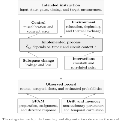
Noise enters between an intended instruction and an observed record through several physically and operationally distinct mechanisms. The categories overlap: for example, crosstalk may produce coherent overrotation, correlated dephasing, or readout error. A trustworthy model declares the system boundary, context, time window, and measured quantity.

Begin with a System Boundary

The word “error” is meaningless until the ideal object and retained degrees of freedom are declared. A microwave pulse can be nearly ideal as a transformation on a multilevel circuit while still being a poor qubit gate because it populates an unwanted level. Photon loss can be an unflagged error in one encoding and a detectable erasure in another. Slow frequency motion can look like a fixed offset during one short experiment and like stochastic dephasing after averaging over many runs.

For an experiment with input label $x$ and outcome $y$, a complete operational model separates preparation, evolution, and measurement:

$$p(y\mid x,t,c) = \operatorname{Tr} \left[ M_{y,t,c}\, \widetilde{\mathcal E}_{t,c} \left( \rho_{x,t,c} \right) \right].$$

The observed probability can change because $\rho_{x,t,c}$ changed, because the process changed, because the measurement changed, or because several changed together. A fit that attributes all discrepancy to “gate noise” may be non-identifiable.

Before assigning an error rate, specify:

• the computational or code subspace;
• the ideal state, gate, channel, instrument, or output distribution;
• the input ensemble and circuit contexts being weighted;
• the time interval over which stationarity is assumed;
• the metric and its operational task;
• whether leakage, loss, postselection, and failed shots are included;
• whether preparation and measurement are trusted or jointly estimated.

There is no context-free scalar called the error rate of a processor.

A Practical Taxonomy

The most useful first division is not “hardware error versus software error.” It is the way an imperfection transforms quantum amplitudes, populations, subspaces, and observed probabilities.

Mechanism	Operational signature	Why it matters
coherent control error	systematic unitary displacement	amplitudes can add coherently with depth
incoherent error	stochastic mixing or irreversible reduced dynamics	purity and distinguishability may decay
relaxation and dephasing	population or phase coherence decays in time	idle and gate durations become resources
leakage or loss	state leaves the declared computational space	qubit-only models and decoders may fail
crosstalk	an operation depends on activity elsewhere	local, independent error assumptions break
SPAM	preparation or readout differs from its declared model	gate estimates and output distributions are biased
drift	process changes during data acquisition	averaging can conceal nonstationarity
correlated noise	faults are statistically or dynamically dependent	long circuits and codes can fail differently from independent models

These categories are not mutually exclusive. A neighboring drive can induce a coherent $ZZ$ phase, heating can increase leakage and relaxation, and slow drift can create temporal correlations that resemble non-Markovian dynamics in reduced data.

Coherent Errors

A coherent error preserves purity when considered on the modeled closed system but implements the wrong unitary. If the target gate is $U$ and the actual gate has a small systematic rotation,

$$\widetilde U = V_\epsilon U, \qquad V_\epsilon = \exp\left( -\frac{i\epsilon G}{2} \right),$$

then $\epsilon$ is an amplitude-level error. Typical causes include pulse-area error, detuning, residual coupling, phase-reference error, uncompensated Stark shifts, and imperfect cancellation of always-on interactions.

Coherent errors are dangerous because repeated aligned amplitudes can add before probabilities are formed. For an identity experiment on $|0\rangle$ with the same unwanted $X$ rotation repeated $L$ times,

$$\begin{aligned} V_\epsilon^L &= \exp\left( -\frac{iL\epsilon X}{2} \right), \\ \Pr(1) &= \sin^2\left( \frac{L\epsilon}{2} \right) \simeq \frac{L^2\epsilon^2}{4}, \end{aligned}$$

when $L|\epsilon|\ll 1$. The quadratic small-$L$ growth is a special aligned case, not a universal law for every coherent circuit. Randomized compiling, changing gate axes, and circuit structure can alter the accumulation.

For a one-qubit Pauli overrotation, the average gate infidelity and diamond distance scale differently:

$$\begin{aligned} r &= 1-F_{\mathrm{avg}} \\ &= \frac{2}{3} \sin^2\left( \frac{\epsilon}{2} \right) \simeq \frac{\epsilon^2}{6}, \\ D_\diamond &= \frac12 \left\| \mathcal V_\epsilon-\mathcal I \right\|_\diamond \\ &= \left| \sin\left( \frac{\epsilon}{2} \right) \right| \simeq \frac{|\epsilon|}{2}. \end{aligned}$$

Thus a small average infidelity can coexist with a much larger worst-case channel distance. This is one reason randomized-benchmarking numbers cannot be compared naively with worst-case fault-tolerance assumptions.

Incoherent Errors and Decoherence

An incoherent effective error maps a pure input to a mixed reduced state or randomly applies different transformations from run to run. It may arise from uncontrolled entanglement with an environment, classical noise averaged over unresolved variables, spontaneous emission, thermal exchange, or deliberately randomized control.

For independent opportunities with fault probability $p$, the probability of at least one fault in $L$ locations is

$$p_{\geq 1} = 1-(1-p)^L \simeq Lp$$

for $Lp\ll 1$. This linear estimate is a bookkeeping approximation. It does not determine the output error because faults can propagate, cancel, be detected, have unequal effects, or be correlated.

Decoherence is the loss of phase coherence in a chosen reduced description due to entanglement with or averaging over uncontrolled degrees of freedom. It is not a synonym for every implementation error. A perfectly isolated but miscalibrated pulse can be wrong without decohering anything; an open-system process can also change populations as well as coherences. Dephasing versus Dissipation develops that distinction.

The coherent/incoherent division is itself model dependent. A slowly varying detuning is approximately a fixed coherent offset within one shot, a random coherent offset across shots, and an apparent dephasing process after ensemble averaging.

Relaxation, Dephasing, and Coherence Times

For a two-level system, $T_1$ conventionally describes longitudinal energy relaxation and $T_2$ describes transverse coherence decay. A Ramsey experiment often reports $T_2^\ast$, which can include slow inhomogeneous broadening and quasistatic frequency variation in addition to faster irreversible processes.

In the restricted weak-coupling, Markovian two-level model with independent pure dephasing,

$$\frac{1}{T_2} = \frac{1}{2T_1} + \frac{1}{T_\phi}, \qquad T_2\leq 2T_1.$$

The relation is a model statement, not a definition valid for arbitrary driven systems, multilevel devices, nonexponential decay, or non-Markovian environments. Decoherence Timescales explains what coherence times measure and when exponential fits are justified.

Coherence times alone do not predict gate performance. A gate may be much shorter than $T_1$ and still suffer control error, crosstalk, leakage, or drive-induced dephasing. Conversely, echo sequences can suppress selected low-frequency noise without changing $T_1$. Report the pulse sequence, fit model, temperature, operating point, and uncertainty along with any $T$ value.

Leakage and Loss

A qubit is usually an encoding inside a larger Hilbert space. Let $P$ project onto the declared computational subspace. For an input $\rho=P\rho P$, the output leakage probability is

$$\begin{aligned} L_{\mathcal E}(\rho) &= \operatorname{Tr} \left[ (I-P)\mathcal E(\rho) \right] \\ &= 1- \operatorname{Tr} \left[ P\mathcal E(\rho) \right]. \end{aligned}$$

Leakage includes population of higher circuit levels, unwanted atomic states, modes outside a photonic encoding, and states outside a code space when that boundary is intended. Loss may be modeled as leakage into an orthogonal vacuum or erasure state, but whether it is flagged is operationally crucial.

Leakage is not equivalent to an ordinary Pauli error:

• later qubit gates may act unpredictably on leaked states;
• a leaked subsystem can remain outside the code for many cycles;
• interactions can spread damage to neighboring qubits;
• apparent return to the code space, called seepage, need not restore the logical state;
• postselecting leaked shots changes the success probability and target task.

Bits, Qubits, Qudits, and Modes owns the encoding hierarchy. Erasure and Loss Channels owns the canonical channel models.

Leakage and Crosstalk owns the QI-facing full-space and retained-branch construction, state and average leakage/seepage/coherence diagnostics, leakage flags, operational locality tests, and context-aware composition; this page retains the broad mechanism taxonomy, accumulation patterns, drift and memory warnings, diagnostics, and engineering response.

Crosstalk

Crosstalk occurs when the realized operation on one subsystem depends on control, state, or measurement activity elsewhere in a way excluded by the intended local model. Operational examples include:

• microwave or optical drive spillover;
• residual $ZZ$ or exchange coupling;
• shared control lines or resonator modes;
• spectator-state-dependent phases;
• simultaneous-gate frequency collisions;
• measurement-induced dephasing of neighbors;
• correlated readout assignments.

The same physical interaction can produce coherent, stochastic, leakage, or SPAM errors. “Crosstalk” identifies the failed independence or locality assumption, not a unique channel.

If an intended parallel layer is $\mathcal G_A\otimes\mathcal G_B$, a context-sensitive implementation generally cannot be written as

$$\widetilde{\mathcal G}_{AB} = \widetilde{\mathcal G}_A \otimes \widetilde{\mathcal G}_B$$

with context-independent local maps. Characterizing each gate in isolation then misses the simultaneous-operation error. Crosstalk is especially consequential for error correction because threshold analyses usually require some form of spatial locality or rapidly decaying correlations.

State-Preparation and Measurement Errors

SPAM abbreviates state-preparation and measurement error. Preparation can have thermal population, imperfect reset, phase error, leakage, or correlations. Measurement can have assignment error, finite efficiency, relaxation during readout, detector memory, correlated resonator response, threshold drift, or disturbance of nearby qubits.

A simple classical assignment model writes

$$\begin{aligned} \widetilde p(y) &= \sum_z A_{yz}\,p_{\mathrm{ideal}}(z), \\ \sum_y A_{yz} &= 1. \end{aligned}$$

where $A_{yz}$ is the probability of reporting $y$ when the latent ideal result is $z$. Inverting an estimated $A$ can mitigate this restricted error model, but it can also amplify sampling noise. The model fails when readout depends on the premeasurement quantum state in an unmodeled way, on simultaneous outcomes, on leakage, or on recent measurement history.

Preparation and measurement are often not separately identifiable from gate data without trusted references or a joint model. Randomized Benchmarking reduces sensitivity of the fitted decay to time-independent SPAM offsets, but it does not make SPAM disappear from the experiment. Gate-set tomography estimates a self-consistent collection of preparations, gates, and measurements, with gauge freedom and model assumptions that must be reported.

SPAM Errors owns the QI-facing preparation-state and operation, POVM/instrument, assignment-license, identifiability, gauge, context-transfer, and validation crosswalk; this page retains the broad mechanism taxonomy, accumulation patterns, diagnostics, and engineering response.

Drift, Correlations, and Memory

Calibration parameters move. Frequencies, amplitudes, phases, temperatures, detector thresholds, optical alignment, magnetic fields, and crosstalk coefficients can vary over minutes, days, or device cycles. If calibration data and application data are collected at different times, a high-quality calibration can be irrelevant to the later workload.

Drift makes the process explicitly time dependent:

$$\widetilde{\mathcal E}_{t_1,c} \neq \widetilde{\mathcal E}_{t_2,c}.$$

Averaging many epochs into one map can fit the mean data while underestimating tails, bursts, and run-to-run uncertainty. Randomizing acquisition order, interleaving references, recording timestamps and calibrations, and repeating on several days help reveal this failure mode.

Noise can also be correlated:

• temporal correlation: a fault changes the probability of later faults;
• spatial correlation: several qubits respond to a shared disturbance;
• context correlation: an error depends on neighboring operations or states;
• cross-layer correlation: preparation, gates, and measurement share a latent cause.

Markovianity is a property of a specified reduced description and time resolution. Long-lived environmental modes, quasistatic offsets, or system-environment correlations can invalidate a memoryless composition model. What Non-Markovian Means owns the formal distinctions; a nonexponential fit alone does not uniquely identify a microscopic memory mechanism.

Markovian and Non-Markovian Noise owns the QI-facing claim ladder from fixed-step composition through CP divisibility and multitime causal breaks, together with drift and boundary confounders; this page retains the broad mechanism taxonomy, accumulation patterns, diagnostics, and engineering response.

Why One Fidelity Number Is Not Enough

Different metrics answer different operational questions. For a target unitary $U$ acting on a $d$-dimensional system, the average gate fidelity is

$$F_{\mathrm{avg}}(\mathcal E,U) = \int d\psi\, \langle\psi| U^\dagger \mathcal E \left( |\psi\rangle\langle\psi| \right) U |\psi\rangle.$$

It averages over pure inputs with the Haar measure. It does not directly bound every entangled input, every circuit context, leakage outside the chosen space, or nonstationary behavior.

The diamond distance

$$D_\diamond(\mathcal E,\mathcal U) = \frac12 \left\| \mathcal E-\mathcal U \right\|_\diamond$$

is a worst-case channel distinguishability measure that permits an entangled ancilla. It has stronger compositional meaning but is harder to estimate experimentally. Other tasks need other quantities:

• leakage and seepage rates for subspace loss;
• assignment matrices and conditional errors for readout;
• unitarity-like measures for coherent content;
• logical error per correction cycle for encoded computation;
• output-distribution distance or observable bias for an application;
• loss, heralding probability, and conditional fidelity for communication.

Fidelity and Trace Distance give the corresponding state-level formulas. A channel metric must be matched to the task and to the assumptions of the experiment used to estimate it.

What Common Diagnostic Tools Establish

No single experiment identifies every noise mechanism. A useful hierarchy moves from components toward the workload:

Diagnostic	Strong use	Important limitation
spectroscopy, Rabi, Ramsey, echo, $T_1$	identify frequencies, control response, and selected time-domain decay	does not predict full multi-gate circuit error
state or process tomography	reconstruct a declared state or process under trusted SPAM	scales poorly and inherits reference errors
gate-set tomography	fit a self-consistent operational gate set	model, stationarity, Markov, and gauge choices matter
randomized benchmarking	estimate a scalable average decay under a randomized gate ensemble	a decay parameter is not automatically worst-case error or workload performance
simultaneous and crosstalk tests	reveal context dependence and correlated response	tests only sampled contexts
circuit or cycle benchmarks	probe compiled layers closer to error-correction or application use	result is workload and compiler dependent
cross-entropy benchmarking	score random-circuit outputs against ideal probabilities	fidelity interpretation needs scrambling and noise assumptions; the score alone does not certify distributional closeness
end-to-end validation	tests the actual protocol and success criterion	may diagnose little about the physical cause

Randomized benchmarking is valuable partly because a decay fit can be robust to constant SPAM offsets. Its interpretation still depends on the sampled gate distribution, compilation, time dependence, leakage, and noise assumptions. Gate-set tomography can expose coherent and context-dependent discrepancies that a single average decay obscures, but it is not assumption free.

A credible characterization campaign combines several rows and checks whether their predictions agree on held-out circuits.

From Characterization to Action

Different interventions solve different problems:

1. Calibration and control engineering reduce the physical error at its source by pulse shaping, better isolation, improved materials, feedback, refocusing, or operating-point choice.
2. Noise tailoring randomizes or symmetrizes selected coherent errors into a form that a decoder or analysis handles more predictably.
3. Error mitigation uses assumptions, modified circuits, and additional samples to reduce bias in selected estimated observables without producing a protected logical state.
4. Quantum error correction encodes information, extracts syndromes, and attempts recovery while preserving the logical state.
5. Fault tolerance constrains the full preparation-gate-measurement architecture so a bounded number of physical faults does not spread into uncontrolled logical failure.

Error Mitigation Overview owns the estimator-level decision among suppression, response correction, extrapolation, cancellation, filtering, encoded correction, or no intervention, including bias, covariance, acceptance, calibration, validation, and total cost; this page retains the device-facing mechanism taxonomy, diagnostic hierarchy, and engineering response.

These levels are complementary, not interchangeable. Zero-noise extrapolation and probabilistic error cancellation can improve expectation-value estimates for sufficiently shallow circuits, but their sampling costs and model sensitivity grow with noise and depth. Error correction consumes qubits, measurements, classical decoding, and time, and succeeds only relative to a noise model and threshold architecture.

Quantum Error Correction and Fault Tolerance begins from a declared physical fault model and routes correctability, syndrome extraction, decoding, fault containment, logical evidence, thresholds, and resources; this page retains device-facing mechanisms, context, correlation, leakage, diagnostics, and engineering response.

Variational Quantum Algorithms develops how bias, estimator variance, drift, and noise-induced concentration alter an adaptive objective landscape and its resource requirements.

The Claims, Hype, and Evidence Standards page explains how to keep component benchmarks, logical demonstrations, and application claims distinct.

A Noise-Budget Workflow

For a real protocol, use the following sequence:

1. Declare the target. Name the ideal channel, distribution, observable, or logical operation.
2. Draw the boundary. List computational, leakage, environmental, control, and measurement degrees of freedom.
3. Inventory locations. Include preparation, gates, idles, routing, resets, measurements, feed-forward, and discarded runs.
4. Classify mechanisms. Separate coherent, stochastic, leakage, loss, SPAM, crosstalk, drift, and correlations where data permit.
5. Choose matched metrics. Use at least one component metric and one end-to-end task metric.
6. Test context and time. Compare isolated with simultaneous operations, short with long sequences, and calibration with later data.
7. Validate predictions. Fit on one circuit set and test on held-out circuits or correction cycles.
8. Attach uncertainty. Include shot uncertainty, fit uncertainty, model discrepancy, and between-run variation.
9. Select an intervention. Suppress, tailor, mitigate, correct, or redesign based on the diagnosed mechanism.
10. Revalidate after compilation. Optimization can reduce depth while changing crosstalk, idle exposure, or coherent cancellation.

An unexplained residual is part of the noise budget. It should not be hidden by renormalizing successful shots or by quoting only the best calibration window.

Common Mistakes

• Calling every discrepancy decoherence.
• Inferring gate fidelity directly from $T_1$ or $T_2$.
• Treating coherent overrotation as an independent stochastic fault with the same one-shot probability.
• Fitting one stationary channel across visible drift without a goodness-of-fit test.
• Ignoring leakage because computational-basis readout maps leaked states to ordinary bit values.
• Measuring gates only in isolation when the workload applies them simultaneously.
• Correcting a readout confusion matrix without propagating calibration and sampling uncertainty.
• Comparing average benchmark infidelity directly with a worst-case fault-tolerance threshold.
• Reporting conditional fidelity after postselection without the acceptance probability.
• Assuming a Markovian channel model because it is convenient to simulate.

Exercises

1. Coherent accumulation

A qubit starts in $|0\rangle$. Each nominal identity cycle applies the same unwanted rotation $\exp(-i\epsilon X/2)$ with $\epsilon=10^{-3}$. Estimate the probability of measuring $1$ after $L=100$ cycles. Compare it with $100$ times the one-cycle probability.

Solution

The exact coherent result is

$$p_{100} = \sin^2(0.05) \simeq 2.50\times 10^{-3}.$$

The one-cycle probability is

$$p_1 = \sin^2(5\times10^{-4}) \simeq 2.50\times10^{-7},$$

so $100p_1\simeq2.50\times10^{-5}$. The aligned coherent error is about one hundred times larger because the rotation angles add before squaring. This comparison applies to the specified repeated-axis experiment; a general circuit can rotate or randomize the error axis.

2. Independent fault bookkeeping

Each of $L=200$ circuit locations has an independent fault probability $p=2\times10^{-4}$. Compute the probability of at least one fault and compare it with $Lp$.

Solution

The exact probability is

$$p_{\geq1} = 1-(1-2\times10^{-4})^{200} \simeq 0.03921.$$

The linear approximation gives

$$Lp=0.04.$$

The approximation is close because $Lp\ll1$. Neither number is automatically the circuit failure probability: some faults may be harmless, detected, corrected, or mutually canceling.

3. Infer a pure-dephasing time

In the simple Markovian two-level model, a device has $T_1=80\,\mu\mathrm{s}$ and $T_2=60\,\mu\mathrm{s}$. Find $T_\phi$. Would $T_2=180\,\mu\mathrm{s}$ be consistent with the same model and $T_1$?

Solution

Using

$$\frac1{T_\phi} = \frac1{T_2} - \frac1{2T_1},$$

gives

$$\frac1{T_\phi} = \frac1{60} - \frac1{160} = \frac1{96}$$

in inverse microseconds. Therefore $T_\phi=96\,\mu\mathrm{s}$.

The model requires $T_2\leq2T_1=160\,\mu\mathrm{s}$. A reported value of $180\,\mu\mathrm{s}$ would be inconsistent with that simple fit model or with the matched interpretation of the two measurements. It would prompt checks of pulse sequences, uncertainties, nonexponential behavior, and whether the quoted quantities describe the same operating condition.

4. Detect leakage with a projector

The computational subspace is spanned by $|0\rangle$ and $|1\rangle$ inside a three-level system. After a gate,

$$\rho' = 0.70|0\rangle\langle0| + 0.25|1\rangle\langle1| + 0.05|2\rangle\langle2|.$$

Find the leakage probability. If the detector reports $|2\rangle$ as bit $1$, what bit probability is observed?

Solution

With

$$P = |0\rangle\langle0| + |1\rangle\langle1|,$$

the leakage is

$$L = 1-\operatorname{Tr}(P\rho') = 0.05.$$

If $|2\rangle$ is assigned to bit $1$, the observed bit-one probability is $0.25+0.05=0.30$. A two-outcome record alone then hides the leakage unless the measurement is separately calibrated to distinguish the third level.

5. Classify a context-dependent error

Gate $X_A$ has low error when run alone. When a measurement pulse is applied to qubit $B$, Ramsey data on $A$ acquire a deterministic phase and the readout assignment probabilities of both qubits become correlated. Which categories apply?

Solution

At least three categories apply:

• crosstalk, because the process on $A$ depends on activity on $B$;
• coherent error, because $A$ acquires a deterministic phase;
• correlated SPAM, because the reported outcomes have joint assignment behavior not captured by independent readout matrices.

Calling the entire effect “measurement noise” would hide the control phase on $A$ and the failed locality assumption.

6. Compare average and worst-case scaling

For a small one-qubit Pauli overrotation, use

$$r\simeq\frac{\epsilon^2}{6}, \qquad D_\diamond\simeq\frac{|\epsilon|}{2}.$$

If randomized benchmarking reports $r=10^{-4}$ and the error is known to be this coherent form, estimate $|\epsilon|$ and $D_\diamond$.

Solution

The angle is

$$|\epsilon| \simeq \sqrt{6r} = \sqrt{6\times10^{-4}} \simeq 2.45\times10^{-2}.$$

Therefore

$$D_\diamond \simeq \frac{|\epsilon|}{2} \simeq 1.22\times10^{-2}.$$

The worst-case distance is more than two orders of magnitude larger than $r$ numerically because the two metrics have different small-angle scaling. The inference depends on knowing that the error is a coherent Pauli overrotation; $r$ alone does not identify the mechanism.

7. Design a validation split

You have time to run $300$ circuits for fitting a noise model and $100$ additional circuits. How should the final $100$ be used to test whether the model predicts the intended workload?

Solution

Keep the final $100$ circuits out of model fitting. Choose them to stress features relevant to the workload that vary from the training set, such as greater depth, simultaneous gates, long idles, different qubit neighborhoods, repeated syndrome-like cycles, and several acquisition times.

Before collecting them, define predictive quantities and tolerances: output probabilities or observables with shot intervals, leakage, and perhaps a distribution distance. Compare predictions with observations and examine residuals versus depth, context, and time. A model that fits the original $300$ circuits but fails systematically on the held-out set has not earned an end-to-end noise claim.

References

• M. A. Nielsen and I. L. Chuang, Quantum Computation and Quantum Information, 10th anniversary edition, Cambridge University Press, 2010, doi:10.1017/CBO9780511976667.
• H.-P. Breuer, E.-M. Laine, J. Piilo, and B. Vacchini, “Colloquium: Non-Markovian dynamics in open quantum systems,” Reviews of Modern Physics 88, 021002 (2016), doi:10.1103/RevModPhys.88.021002.
• E. Magesan, J. M. Gambetta, and J. Emerson, “Scalable and robust randomized benchmarking of quantum processes,” Physical Review Letters 106, 180504 (2011), doi:10.1103/PhysRevLett.106.180504.
• T. Proctor, K. Rudinger, K. Young, M. Sarovar, and R. Blume-Kohout, “What randomized benchmarking actually measures,” Physical Review Letters 119, 130502 (2017), doi:10.1103/PhysRevLett.119.130502.
• R. Kueng, D. M. Long, A. C. Doherty, and S. T. Flammia, “Comparing experiments to the fault-tolerance threshold,” Physical Review Letters 117, 170502 (2016), doi:10.1103/PhysRevLett.117.170502.
• C. J. Wood and J. M. Gambetta, “Quantification and characterization of leakage errors,” Physical Review A 97, 032306 (2018), doi:10.1103/PhysRevA.97.032306.
• M. Sarovar, T. Proctor, K. Rudinger, K. Young, E. Nielsen, and R. Blume-Kohout, “Detecting crosstalk errors in quantum information processors,” Quantum 4, 321 (2020), doi:10.22331/q-2020-09-11-321.
• K. Rudinger, T. Proctor, D. Langharst, M. Sarovar, K. Young, and R. Blume-Kohout, “Probing context-dependent errors in quantum processors,” Physical Review X 9, 021045 (2019), doi:10.1103/PhysRevX.9.021045.
• K. Temme, S. Bravyi, and J. M. Gambetta, “Error mitigation for short-depth quantum circuits,” Physical Review Letters 119, 180509 (2017), doi:10.1103/PhysRevLett.119.180509.
• J. Preskill, “Quantum computing in the NISQ era and beyond,” Quantum 2, 79 (2018), doi:10.22331/q-2018-08-06-79.

See Also

• Common Noise Models
• Pauli Noise and Depolarizing Channels
• Dephasing and Amplitude Damping
• Device Characterization
• Randomized Benchmarking
• Cycle Benchmarking
• Cross-Entropy Benchmarking
• Noise Simulation
• Quantum Channels and Noise
• What Is Decoherence?
• Dephasing versus Dissipation
• What Non-Markovian Means
• Density Operators for Quantum Information
• Circuit Model
• Quantum Software Stack
• Error-Aware Compilation
• Claims, Hype, and Evidence Standards
• Bits, Qubits, Qudits, and Modes