Pauli Noise and Depolarizing Channels
A Pauli-noise model is useful only after its probability object, frame, circuit location, time step, and independence assumptions have been fixed. This page develops the computational crosswalk from that record to Pauli-transfer eigenvalues, repeated-channel composition, Clifford transport, syndrome probabilities, and logical recovery classes. It also gives a precise qubit depolarizing-convention ledger and tests what is lost when a physical process is replaced by a Pauli or isotropic surrogate. The aim is not to infer a microscopic mechanism from a fitted law, but to make every modeling and propagation claim reproducible.
Required background. Quantum Channels for QI supplies transfer coordinates, representation conventions, channel composition, and finite physicality checks. Stabilizer Formalism supplies Pauli groups, Clifford conjugation, stabilizer syndromes, and logical cosets.
Helpful background. Common Noise Models supplies the broader device-facing model and parameter ledger. Noise in Quantum Information supplies mechanism, accumulation, context, and diagnostic language.
Pauli Noise as a Computational Model
Section titled “Pauli Noise as a Computational Model”Stochastic Pauli events and the unread map
Section titled “Stochastic Pauli events and the unread map”Fix the phase-free one-qubit label order
In a sampled description, a classical random variable takes value with probability , and the state in that trajectory is transformed as . If the classical label is not retained, the operational channel is the ensemble average
The trajectory and the unread map are two descriptions of the same declared stochastic experiment, but they support different calculations. A simulator may sample labels without constructing a density operator; a prediction for an unconditioned observable averages over those samples. Conversely, writing a Pauli channel does not prove that a device produced a definite hidden Pauli at each run. It states an effective completely positive trace-preserving map and one stochastic realization of that map. Nielsen and Chuang give the standard operator and circuit language for this distinction, while Watrous develops its channel-theoretic form.
Why the model is computationally useful
Section titled “Why the model is computationally useful”Pauli labels form a finite group after global phases are discarded. Composition therefore reduces to a classical convolution, and the group characters turn that convolution into componentwise multiplication. Clifford gates permute Pauli labels under conjugation. Stabilizer measurements map each label to a binary syndrome, after which a chosen recovery partitions labels into logical classes. Each step is finite and auditable.
These facts explain why Pauli models are central to stabilizer-circuit analysis. Aaronson and Gottesman show how the Clifford–Pauli closure supports efficient trajectory simulation, and Gottesman’s stabilizer-code treatment explains the syndrome and coset structure used below. Efficiency, however, is conditional on the model: a compact Pauli trajectory need not preserve the interference, leakage, temporal memory, or continuously valued coherent parameters of the underlying device.
What this page owns
Section titled “What this page owns”The computational object here is a declared probability law and its pushforwards. Formal Kraus, Choi, complete-positivity, and twirl derivations remain at Pauli Channels; the dimension-dependent isotropic family remains at Depolarizing Channel. This page instead asks whether the law is normalized, which convention its parameters use, how it composes, how ideal gates transport its labels, and what syndrome or logical distribution it predicts.
That ownership boundary matters experimentally. A fitted Pauli law can be an excellent task-specific surrogate without being a microscopic account. Geller and Zhou analyze when Pauli-twirled models can be useful for fault-tolerant estimates and why coherent structure can still change the answer. The correct claim is therefore always attached to a circuit family, observable, parameter range, and validation domain.
Freeze the Pauli-Noise Record
Section titled “Freeze the Pauli-Noise Record”System, Pauli frame, and circuit location
Section titled “System, Pauli frame, and circuit location”Begin a calculation with a record rather than a bare number. State the Hilbert-space factorization and the phase-free Pauli basis on each factor. State whether , , and are laboratory axes, logical-frame axes, or axes after an ideal target has been removed. For a gate error, decide whether the noise is placed before the gate, after it, or written as an error channel relative to the ideal operation. These choices determine which Pauli label is transported.
Circuit location is part of the random variable. An before a Hadamard becomes a after that Hadamard, whereas an inserted after it does not. Across a controlled-NOT, a control- spreads to the target while a target- spreads to the control. Omitting location can therefore turn the same printed probability vector into different joint laws later in a circuit.
Probability law, correlations, and time step
Section titled “Probability law, correlations, and time step”For one qubit, record the entire vector in the declared order. For qubits, record the joint law rather than only its one-qubit marginals. If the law is assumed to factorize, say so explicitly. If it varies by gate type, layer, qubit, direction, or classical context, those labels belong in the model record too.
Also freeze the time step: one primitive gate, one compiled cycle, one idle window, one error-correction round, or another named interval. Probabilities attached to different intervals cannot be composed until the intervening ideal operations and correlations have been specified. A memoryless assumption means successive labels are independently drawn from the stated step law. It is stronger than observing a similar average decay at several depths.
Observable, validation domain, and approximation claim
Section titled “Observable, validation domain, and approximation claim”Name the output being predicted: a Pauli expectation, a syndrome histogram, an acceptance probability, a decoder input, or a logical failure probability. Then state the circuit family, depths, input states, measurement axes, device contexts, and epochs on which the model was fitted and checked. A dataset label may index a frozen context, but it does not replace the physical description of that context.
Finally, phrase the approximation as a bounded claim. “This cycle-level Pauli law predicts these held-out syndrome frequencies within the stated uncertainty” is testable. “The noise is Pauli” is not, unless the experiment has excluded relevant alternatives. Chen and collaborators show that learning Pauli noise has nontrivial identifiability structure; a model record must expose the assumptions under which particular parameters are learnable.
Single-Qubit Pauli Channels
Section titled “Single-Qubit Pauli Channels”Probability simplex and channel action
Section titled “Probability simplex and channel action”For the fixed order , write
The four nonnegative weights occupy a three-dimensional probability simplex. Its vertices are the four Pauli conjugations. The identity vertex leaves every state unchanged; the other vertices are still unitary channels, not maximally noisy maps. Mixtures in the interior describe uncertainty over these conjugations.
This probability statement is already a physicality certificate: the displayed operator-sum realization is trace preserving and completely positive. The converse statements below require more care. They apply only after the candidate map has been declared trace preserving, unital, and diagonal in this exact Pauli basis. A generic real diagonal-looking array with the correct identity entry need not represent a completely positive quantum channel.
Bloch and Pauli-transfer eigenvalues
Section titled “Bloch and Pauli-transfer eigenvalues”Write . Pauli conjugation preserves its own Bloch component and reverses the other two. Therefore
with
Equivalently, and , with analogous equations for and . These eigenvalues do not depend on whether the Pauli basis is normalized, provided the same convention is used at input and output. They directly encode axis-resolved contraction and sign reversal. Negative is allowed: the corresponding Bloch component is reversed as well as contracted.
Invert eigenvalues back to probabilities
Section titled “Invert eigenvalues back to probabilities”The inverse Walsh–Hadamard transform is
For a trace-preserving, unital, Pauli-diagonal qubit map in the stated order, nonnegativity of these four numbers is necessary and sufficient for complete positivity. Thus the complete-positive region in is the tetrahedron whose vertices correspond to . The larger cube maps the Bloch ball into itself for a diagonal unital map, but it is not the CPTP region. For example, lies in the cube and gives a negative inverse probability.
This distinction is an efficient audit of fitted eigenvalues. Finite-sample estimates can fall outside the tetrahedron; one must then report uncertainty or use a constrained estimator, not silently clip each eigenvalue to the cube. The formal geometry and its complete-positivity interpretation are developed at the canonical Pauli-channel owner.
Depolarizing Conventions and Conversion
Section titled “Depolarizing Conventions and Conversion”Replacement, total-Pauli, shrink, and infidelity parameters
Section titled “Replacement, total-Pauli, shrink, and infidelity parameters”Two common qubit formulas attach different meanings to their displayed parameter. The total-nonidentity-Pauli convention is
On the range where is a literal replacement probability, the same channel is
Its common Bloch and nonidentity-Pauli eigenvalue is . For an identity target and the maximally mixed qubit channel input,
Here is channel entanglement fidelity relative to the identity, evaluated using a maximally entangled purification of the maximally mixed input. It is not an input-independent state fidelity. For a nonidentity target, the target must first be removed consistently so that these are parameters of the error channel. The average-fidelity relation is a standard consequence of the channel-fidelity identity presented by Nielsen.
| quantity | symbol | defining expression | identity limit | allowed or shared range | common convention failure |
|---|---|---|---|---|---|
| identity branch weight | Calling it the Bloch shrink | ||||
| total nonidentity Pauli probability | Calling the replacement strength | ||||
| replacement strength | Literal mixture only for | Treating as a probability | |||
| common Pauli-transfer or Bloch shrink | for the Pauli mixture | Excluding physical negative shrink factors | |||
| entanglement infidelity | in the declared family | Using it as every input-state infidelity | |||
| average infidelity | for the Pauli mixture | Setting |
The shared range and negative shrink factors
Section titled “The shared range and negative shrink factors”The literal replacement form and the Pauli mixture coincide for , equivalently and . At , the output is for every input: and . This is the completely depolarizing point.
The Pauli mixture remains CPTP beyond that point. At , it applies , , or with equal probability, has , and corresponds algebraically to . That is a conversion coordinate, not a literal mixing probability. Negative shrink does not mean negative probability; it means that all three Bloch axes reverse while shrinking. The dimension-dependent CP range and generalized-Pauli representation belong to the formal depolarizing-channel page.
Repetition uses contraction, not linear probability
Section titled “Repetition uses contraction, not linear probability”For independent repetitions of the same memoryless depolarizing map, each application multiplies every traceless Pauli component by . After repetitions,
Adding counts “at least one event” incorrectly because two Pauli events can cancel phase-free or combine into a third Pauli. The linear rule is only a first-order small-error approximation, and even then its remainder depends on the convention. The semigroup-like quantity is the contraction, or when , not the finite-step error probability.
Pauli-Transfer Eigenvalues and Composition
Section titled “Pauli-Transfer Eigenvalues and Composition”Convolution of Pauli labels
Section titled “Convolution of Pauli labels”Let describe the first Pauli event and the second. Discarding the irrelevant global phase, their product is another Pauli label. The probability of the resulting label is the Klein-four convolution
For example,
because equal nonidentity labels square to identity up to phase. The component receives , , , and . This gives a direct probability-space calculation whose normalization follows by summing over all products.
Convolution is commutative for phase-free one-qubit labels, even though the Pauli matrices themselves can anticommute: the discarded phase is the only order dependence. Once ideal non-Clifford gates or frame changes intervene, however, the effective error labels need not remain in this group and a bare convolution is no longer justified.
Transfer eigenvalues multiply
Section titled “Transfer eigenvalues multiply”The three sign characters used in the forward transform diagonalize convolution. If and are the eigenvalues of two Pauli channels, then
Thus one can compose in probability space or multiply eigenvalues and invert. Agreement of the two paths is a strong finite check on order and sign conventions. If every nonidentity eigenvalue is nonzero, the linear superoperator has a mathematical inverse, but that inverse is generally not a CPTP channel. A Pauli channel has a CPTP inverse only at a unitary Pauli vertex: otherwise a physical inverse would have to undo irreversible mixing.
For an -fold homogeneous step, . Anisotropic channels retain three different decay factors. Replacing them by one depolarizing shrink discards axis dependence, even when an average-fidelity scalar is preserved.
Frame changes and noncommuting ideal gates
Section titled “Frame changes and noncommuting ideal gates”Let an error occur before an ideal unitary . Moving the error to the output changes it to . For a Clifford , this is another Pauli up to phase and the probability law is permuted. For a generic non-Clifford, the conjugated operator need not be a Pauli, so the Pauli family is not closed under transport.
Even inside the Clifford group, an anisotropic channel cannot be moved through a gate without relabeling its probabilities. A Hadamard exchanges and and reverses only by an irrelevant sign, so its action swaps and . Controlled-NOT can change error weight. Consequently a composition statement must name the ideal gates, the direction of transport, and whether labels are expressed in the incoming or outgoing frame.
Multiqubit Distributions and Correlations
Section titled “Multiqubit Distributions and Correlations”Joint Pauli-string laws
Section titled “Joint Pauli-string laws”For qubits, let denote phase-free strings. A Pauli channel is specified by a joint law
Its transfer eigenvalue on a Pauli string is the character transform
where for commuting strings and for anticommuting strings. The inverse is
This is the multiqubit Walsh–Hadamard transform. Composition again becomes phase-free group convolution, and every multiplies. The representation has independent real parameters, so exact algebraic simplicity does not by itself make a general correlated law statistically or computationally small.
Independence is a factorization assumption
Section titled “Independence is a factorization assumption”An independent local law has
Then its character eigenvalues factorize as well. This can reduce storage and sampling cost dramatically, but it is an assumption about the joint distribution, not a consequence of having measured each marginal. Common-mode fluctuations, residual couplings, shared control, transport, and circuit conditioning can correlate faults while leaving every one-qubit marginal unchanged.
Local and global depolarizing models also differ. If each qubit experiences the same local shrink , a weight- Pauli observable has eigenvalue . A global depolarizing channel on the -dimensional register instead assigns one common eigenvalue to every nonidentity Pauli string. Matching a few weight-one decays cannot identify which model governs high-weight observables.
Weight, locality, bias, and correlated tails
Section titled “Weight, locality, bias, and correlated tails”Useful structured models declare which features they retain: support geometry, string weight, bias, gate location, or long correlated tails. A low mean weight does not exclude rare high-weight events, and those events can dominate a code’s logical failure. One-qubit marginals constrain only sums of joint probabilities.
| model or use | probability object | structure retained | exact task | principal falsifier | canonical boundary |
|---|---|---|---|---|---|
| single-qubit biased Pauli channel | axis bias | one-location expectations | inconsistent held-out axis decay | Formal Pauli-channel theory stays with its owner | |
| independent local Pauli model | product of local laws | qubit dependence without correlations | sampling and low-weight prediction | connected multiqubit statistics | Factorization must be declared |
| correlated multiqubit Pauli model | joint string law | spatial and string correlations | syndrome or observable pushforward | missing correlated tails | Marginals do not determine the joint law |
| circuit-location Pauli model | law conditioned on location | gate and layer context | circuit-level propagation | context-dependent residuals | Placement and frame are part of the model |
| depolarizing baseline | one common shrink | isotropic contraction | scalar baseline and repetition | unequal Pauli-axis decays | Dimension-dependent family stays with its owner |
| Pauli-twirled surrogate | diagonal transfer terms | original Pauli diagonal | compare a twirled observable | sensitivity to removed coherences | It describes an ideal average |
| randomized-compiled ensemble | distribution over dressed circuits | compilation and sampling contract | ensemble-averaged prediction | randomizer or gate dependence | It is not the bare circuit |
| logical effective Pauli model | distribution over logical classes | code and recovery dependence | logical-level propagation | recovery- or circuit-dependent mismatch | Decoder algorithms stay with their owner |
The choice among these rows is driven by the observable, not by a universal hierarchy of realism. A depolarizing baseline can be adequate for a scalar decay and inadequate for a biased-code estimate. A correlated string model can be exact for one cycle yet fail across cycles if temporal memory was omitted.
Clifford Propagation and Stabilizer Simulation
Section titled “Clifford Propagation and Stabilizer Simulation”Clifford conjugation transports Pauli labels
Section titled “Clifford conjugation transports Pauli labels”A Clifford circuit acts by
and permutes phase-free Pauli strings. Therefore a probability mass at is transported to its conjugate label without changing its value. Sequential independent location-dependent laws can be transported into a common output frame and then convolved; correlated locations instead require propagating their declared joint law. The procedure is exact for the declared Pauli errors, dependence assumptions, and ideal Clifford gates.
Generator rules suffice. Hadamard exchanges and ; the phase gate maps to and fixes up to phase. For controlled-NOT with control and target , , , while and remain on their original qubits. Stating control, target, ordering, and error location prevents the most common propagation mistakes.
Stabilizer trajectories and sampled mixtures
Section titled “Stabilizer trajectories and sampled mixtures”In one trajectory, sample a Pauli label at each declared location, propagate it through subsequent Clifford gates, and update the stabilizer state or frame. Repeating trajectories estimates an ensemble observable without storing the full mixed density operator. Aaronson and Gottesman’s tableau algorithm supplies the efficient ideal Clifford backbone; Pauli sampling adds classical randomness around it.
Alternatively, one may propagate an exact probability distribution over labels. That preserves the mixture without Monte Carlo error but can require exponentially many strings. Structured factorization or sparse support may help, provided those structures remain valid under the circuit. Stabilizer Simulation owns the data structures, algorithms, detector streams, performance choices, and run-validation workflow.
What efficient simulation does not certify
Section titled “What efficient simulation does not certify”An efficient trajectory code certifies neither the input model nor its adequacy. It may exactly simulate the wrong effective channel. It also does not turn coherent rotations, amplitude damping, leakage, or non-Markovian memory into stochastic Pauli events. Those require either a richer simulator or a separately justified approximation.
Likewise, a sampled stabilizer trajectory is not generally an observable microscopic history. Different stochastic decompositions can represent the same unread channel, and process data may identify only equivalence classes. The validation question is whether the predicted distributions agree with held-out data relevant to the task, including uncertainty and context.
Syndrome and Logical Pushforwards
Section titled “Syndrome and Logical Pushforwards”Syndromes are a many-to-one pushforward
Section titled “Syndromes are a many-to-one pushforward”For stabilizer generators , define a syndrome bit when anticommutes with and when it commutes. The syndrome distribution is the classical pushforward
Many distinct physical errors share the same syndrome. Stabilizers themselves have trivial syndrome, and multiplying an error by a stabilizer preserves its syndrome. Thus syndrome data can constrain sums of probabilities without identifying individual strings. Flammia and O’Donnell formulate Pauli error estimation as a population-recovery problem, illustrating why the accessible probability combinations depend on the experiment.
Recovery partitions logical cosets
Section titled “Recovery partitions logical cosets”Choose a recovery for every syndrome. After an error , the corrected operator is . It has trivial syndrome and therefore acts, modulo stabilizers, as a logical Pauli class . The logical distribution is
Changing the recovery can change this partition and hence the logical failure probability, even if the physical law and syndrome histogram are fixed. Decoders owns how a recovery or logical class is inferred from data; the present calculation assumes that rule is already frozen.
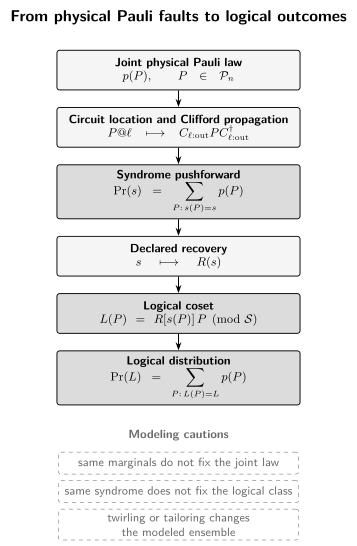
A declared joint law is transported to a circuit location, pushed forward to syndromes, combined with a chosen recovery, and aggregated into logical cosets. Marginals, syndromes, and twirled ensembles each discard different information.
Three-Qubit Codes owns the repetition-code codewords, checks, ideal recovery, and bit-/phase-flip limitations; this page retains only the frozen Pauli-law-to-syndrome-and-logical-class pushforward.
Five-Qubit Code owns the exact five-qubit residual-class enumerator and finite independent-depolarizing polynomial for its declared fixed decoder; this page retains the channel law, independence and correlation assumptions, and syndrome-to-logical pushforward conventions.
Shor Code owns the exact nine-qubit residual-class enumerator and finite fixed-decoder polynomial for its separated recovery; this page retains probability-law, independence and correlation, convention, and syndrome-to-logical pushforward audits.
Steane Code owns the exact seven-qubit residual-class enumerator and finite independent-depolarizing polynomial for its declared fixed decoder; this page retains probability-law, independence and correlation, convention, and syndrome-to-logical pushforward audits.
For a concrete audit, use the three-qubit repetition code with
syndrome order , and bit for anticommutation. Choose , , , and . At independent bit-flip probability , the complete probability pushforward is:
| physical error | probability | syndrome | chosen recovery | resulting logical class |
|---|---|---|---|---|
| logical | ||||
| logical | ||||
| logical | ||||
| logical | ||||
| logical | ||||
| logical | ||||
| logical | ||||
| logical |
Physical, detection, and logical rates differ
Section titled “Physical, detection, and logical rates differ”Three probabilities answer three different questions:
For the table, they are respectively , , and . The difference between the first two is the undetected event. The logical rate includes the three weight-two patterns and , but excludes every corrected weight-one pattern. None of these rates determines either of the others without the code, circuit, full joint law, and recovery.
The separation is not merely semantic. Beale and collaborators show how error correction can suppress coherent components in an effective logical description, but that result does not identify a universal mapping from physical infidelity to logical failure. Why Quantum Error Correction Is Possible develops the coding principle; a quantitative prediction still requires the declared pushforward.
Twirling, Tailoring, and Approximation Boundaries
Section titled “Twirling, Tailoring, and Approximation Boundaries”Pauli twirling removes off-diagonal process terms
Section titled “Pauli twirling removes off-diagonal process terms”For an -qubit channel , its ideal Pauli twirl is
In a fixed Pauli-transfer representation, this average removes off-diagonal terms and preserves the diagonal. The result is Pauli diagonal, subject to the target and frame convention used to define the error channel. It need not be depolarizing because the surviving diagonal entries may differ.
An ideal Haar twirl, or an exact unitary 2-design with the same second moment, additionally enforces isotropy and yields the corresponding depolarizing channel. Dankert and collaborators establish the relevant exact and approximate 2-design framework. The scalar fixed by such a twirl can preserve average fidelity while other operational distances and circuit responses change.
Randomized compiling tailors an ensemble
Section titled “Randomized compiling tailors an ensemble”Randomized compiling inserts and compiles random gates so that the implemented distribution over dressed circuits has a tailored effective noise description. Wallman and Emerson give the theoretical protocol and its assumptions. Hashim and collaborators demonstrate a superconducting-processor implementation, including experimental details that matter when interpreting the effective ensemble.
This operational procedure is not identical to applying an abstract twirl to a fixed channel. Finite sampling, imperfect randomizers, gate dependence, compilation choices, and correlations can alter the dressed ensemble and its residual corrections. The averaging unit may be a gate, cycle, circuit, or dataset; it must be stated. “Randomized compiled” therefore names a protocol and ensemble, not a guarantee that each bare physical fault was an independent Pauli draw.
Twirled and bare circuits answer different questions
Section titled “Twirled and bare circuits answer different questions”A twirled surrogate predicts the ideal average specified by the twirl. A randomized-compiled experiment predicts an empirical ensemble under its sampling and compilation contract. A bare circuit predicts the unrandomized implementation. Agreement for one of these objects does not automatically transfer to the others.
Average infidelity is particularly incomplete. Coherent and stochastic channels can share it while having different depth dependence or logical effects. Geller and Zhou exhibit the stakes for fault-tolerant modeling, and randomized-benchmarking methods deliberately compress behavior into decay summaries. Randomized Benchmarking owns that protocol and its interpretation. A defensible approximation audit compares the exact observable of interest across the bare data and the proposed surrogate rather than inferring adequacy from one matched scalar.
Fit and Falsify a Pauli Model
Section titled “Fit and Falsify a Pauli Model”Estimate only identifiable parameters
Section titled “Estimate only identifiable parameters”Choose measurements whose probabilities depend on the requested Pauli coordinates. Single-axis preparations and measurements can expose axis contractions, while richer circuit ensembles can probe multiqubit characters or location dependence. Flammia and Wallman develop efficient Pauli-channel estimation, and Harper, Flammia, and Wallman show how noise learning can exploit structured circuit data. Erhard and collaborators use cycle benchmarking to characterize large cycles through Pauli-error information relevant to compiled operations.
The experiment may identify transfer eigenvalues, ratios, or equivalence classes more directly than every . SPAM nuisance parameters, gauge freedoms, finite samples, and exponentially many correlated strings limit reconstruction. Chen and collaborators formalize learnability constraints; those constraints should shape the requested output before data are collected. Physicality must be imposed jointly through nonnegative inverse probabilities, not coordinatewise after estimation.
Hold out axes, depths, contexts, and epochs
Section titled “Hold out axes, depths, contexts, and epochs”Fit and validation data should be separated along dimensions that could reveal model failure. Hold out at least one Pauli axis when testing isotropy, depths beyond those used in a decay fit when testing memoryless repetition, and circuit contexts when testing gate independence. Repeat across calibration epochs when stationarity is assumed. For multiqubit laws, include connected statistics or syndromes sensitive to correlations rather than only one-qubit marginals.
Report residuals with uncertainty and propagate parameter uncertainty to the final task quantity. A model that predicts mean observables but misses tails may be adequate for calibration and inadequate for logical-risk estimation. A law fitted at one cycle granularity should not be reinterpreted at a primitive-gate granularity without a composition model.
Failure signatures that require a richer model
Section titled “Failure signatures that require a richer model”Unequal fitted axis contractions falsify an isotropic depolarizing model but may still support a biased Pauli channel. Oscillatory or strongly nonexponential depth dependence suggests coherent evolution, drift, leakage, or temporal memory. Context-dependent residuals challenge a location-independent law. Connected syndromes or parity statistics challenge independent local sampling. Inverse-transform probabilities that remain negative beyond statistical uncertainty challenge the Pauli-diagonal hypothesis or the representation calibration.
No single signature uniquely diagnoses a mechanism. The response is to enlarge the candidate family and design discriminating measurements, not to rename the discrepancy. Common Noise Models provides placement rules and model-specific falsifiers; the effective Pauli crosswalk resumes only after a richer or narrower probability object has been declared.
Three Reproducible Finite Audits
Section titled “Three Reproducible Finite Audits”Audit 1 — Transform probabilities and transfer eigenvalues
Section titled “Audit 1 — Transform probabilities and transfer eigenvalues”Take and in order . Both vectors are normalized and nonnegative. The forward transform gives
Phase-free convolution gives
Independently multiplying transfer eigenvalues gives ; the inverse transform returns the same convolution vector. This asymmetric example catches an accidental exchange of and , a sign error in the character table, or a convolution routine that retains Pauli phases.
Audit 2 — Compose and repeat a depolarizing model
Section titled “Audit 2 — Compose and repeat a depolarizing model”Set the total nonidentity Pauli probability to . The ledger gives , , , and . Five identical memoryless repetitions yield
The composed total Pauli probability is not . Multiplying accounts for cancellations and for products of distinct Pauli labels; adding does neither. The example also separates the per-step entanglement infidelity from the five-step average infidelity .
Audit 3 — Push independent and correlated faults through a code
Section titled “Audit 3 — Push independent and correlated faults through a code”The repetition-code table gives syndrome probabilities in order . Hence the nonzero-syndrome probability is , the probability of at least one physical is , and the logical- probability is .
Now replace independence by the all-or-none law and . Every qubit still has marginal probability , yet the syndrome is always and the logical- probability is . Equal marginals therefore determine neither the joint law nor its logical pushforward. The following dependency-free program recomputes all three audits from primitive inputs and fails hard at absolute tolerance .
"use strict";
const tolerance = 1e-12;const assert = (condition, message) => {  if (!condition) throw new Error(message);};const assertClose = (actual, expected, message) => {  assert(Math.abs(actual - expected) <= tolerance, `${message}: ${actual} != ${expected}`);};const assertVector = (actual, expected, message) => {  assert(actual.length === expected.length, `${message}: length`);  actual.forEach((value, k) => assertClose(value, expected[k], `${message}[${k}]`));};const assertLabels = (actual, expected, message) => {  assert(actual.length === expected.length, `${message}: length`);  actual.forEach((value, k) => assert(value === expected[k], `${message}[${k}]: ${value} != ${expected[k]}`));};const normalizedNonnegative = (probabilities, name) => {  probabilities.forEach((value, k) => assert(value >= 0, `${name}[${k}] is negative`));  assertClose(probabilities.reduce((sum, value) => sum + value, 0), 1, `${name} normalization`);};
const toEigenvalues = ([pI, pX, pY, pZ]) => [  pI + pX - pY - pZ,  pI - pX + pY - pZ,  pI - pX - pY + pZ,];const fromEigenvalues = ([lx, ly, lz]) => [  (1 + lx + ly + lz) / 4,  (1 + lx - ly - lz) / 4,  (1 - lx + ly - lz) / 4,  (1 - lx - ly + lz) / 4,];const productTable = [  [0, 1, 2, 3],  [1, 0, 3, 2],  [2, 3, 0, 1],  [3, 2, 1, 0],];const convolve = (left, right) => {  const result = [0, 0, 0, 0];  for (let a = 0; a < 4; a += 1) {    for (let b = 0; b < 4; b += 1) {      result[productTable[a][b]] += left[a] * right[b];    }  }  return result;};
const pauliP = [0.70, 0.10, 0.05, 0.15];const pauliQ = [0.80, 0.05, 0.10, 0.05];normalizedNonnegative(pauliP, "p");normalizedNonnegative(pauliQ, "q");const lambdaP = toEigenvalues(pauliP);const lambdaQ = toEigenvalues(pauliQ);assertVector(lambdaP, [0.60, 0.50, 0.70], "lambda(p)");assertVector(lambdaQ, [0.70, 0.80, 0.70], "lambda(q)");assertVector(fromEigenvalues(lambdaP), pauliP, "inverse p");assertVector(fromEigenvalues(lambdaQ), pauliQ, "inverse q");const probabilityComposition = convolve(pauliP, pauliQ);const lambdaComposition = lambdaP.map((value, k) => value * lambdaQ[k]);const transformComposition = fromEigenvalues(lambdaComposition);assertVector(lambdaComposition, [0.42, 0.40, 0.49], "lambda(p*q)");assertVector(probabilityComposition, [0.5775, 0.1325, 0.1225, 0.1675], "p*q");assertVector(transformComposition, probabilityComposition, "two composition paths");normalizedNonnegative(probabilityComposition, "p*q");
const pauliProbability = 0.12;const replacementStrength = 4 * pauliProbability / 3;const eta = 1 - replacementStrength;const entanglementInfidelity = pauliProbability;const averageInfidelity = 2 * pauliProbability / 3;assertClose(replacementStrength, 0.16, "q");assertClose(eta, 0.84, "eta");assertClose(entanglementInfidelity, 0.12, "1-Fe");assertClose(averageInfidelity, 0.08, "r");const eta5 = eta ** 5;const replacement5 = 1 - eta5;const pauli5 = 3 * replacement5 / 4;const average5 = replacement5 / 2;assertClose(eta5, 0.4182119424, "eta5");assertClose(replacement5, 0.5817880576, "q5");assertClose(pauli5, 0.4363410432, "p5");assertClose(average5, 0.2908940288, "r5");assert(Math.abs(pauli5 - 5 * pauliProbability) > tolerance, "linear probability was not rejected");
const labels = ["III", "XII", "IXI", "IIX", "XXI", "XIX", "IXX", "XXX"];const bits = labels.map((label) => [...label].map((letter) => Number(letter === "X")));const syndrome = ([x1, x2, x3]) => `${x1 ^ x2}${x2 ^ x3}`;const recoveries = {  "00": [0, 0, 0],  "10": [1, 0, 0],  "11": [0, 1, 0],  "01": [0, 0, 1],};const recoveryNames = { "00": "I", "10": "X1", "11": "X2", "01": "X3" };const logicalClass = (errorBits) => {  const s = syndrome(errorBits);  const corrected = errorBits.map((bit, k) => bit ^ recoveries[s][k]);  if (corrected.every((bit) => bit === 0)) return "I";  if (corrected.every((bit) => bit === 1)) return "X";  throw new Error(`invalid corrected pattern ${corrected.join("")}`);};const bitFlipProbability = 0.1;const independent = bits.map((pattern) => {  const weight = pattern.reduce((sum, bit) => sum + bit, 0);  return bitFlipProbability ** weight * (1 - bitFlipProbability) ** (3 - weight);});assertVector(independent, [0.729, 0.081, 0.081, 0.081, 0.009, 0.009, 0.009, 0.001], "pattern probabilities");normalizedNonnegative(independent, "independent law");assertLabels(  bits.map((pattern) => syndrome(pattern)),  ["00", "10", "11", "01", "01", "11", "10", "00"],  "pattern syndromes",);assertLabels(  bits.map((pattern) => recoveryNames[syndrome(pattern)]),  ["I", "X1", "X2", "X3", "X3", "X2", "X1", "I"],  "chosen recoveries",);assertLabels(  bits.map((pattern) => logicalClass(pattern)),  ["I", "I", "I", "I", "X", "X", "X", "X"],  "pattern logical classes",);const syndromeOrder = ["00", "10", "11", "01"];const syndromeProbabilities = syndromeOrder.map((value) => independent.reduce(  (sum, probability, k) => sum + (syndrome(bits[k]) === value ? probability : 0),  0,));assertVector(syndromeProbabilities, [0.73, 0.09, 0.09, 0.09], "syndrome probabilities");const detectionProbability = syndromeProbabilities.slice(1).reduce((sum, value) => sum + value, 0);const physicalProbability = 1 - independent[0];const logicalProbability = independent.reduce(  (sum, probability, k) => sum + (logicalClass(bits[k]) === "X" ? probability : 0),  0,);assertClose(detectionProbability, 0.27, "nonzero syndrome");assertClose(physicalProbability, 0.271, "at least one physical X");assertClose(logicalProbability, 0.028, "logical X");
const correlated = [0.9, 0, 0, 0, 0, 0, 0, 0.1];normalizedNonnegative(correlated, "all-or-none law");for (let qubit = 0; qubit < 3; qubit += 1) {  const independentMarginal = independent.reduce(    (sum, probability, k) => sum + probability * bits[k][qubit],    0,  );  const marginal = correlated.reduce((sum, probability, k) => sum + probability * bits[k][qubit], 0);  assertClose(independentMarginal, 0.1, `independent marginal ${qubit}`);  assertClose(marginal, 0.1, `correlated marginal ${qubit}`);  assertClose(marginal, independentMarginal, `matched marginal ${qubit}`);}const correlatedDetection = correlated.reduce(  (sum, probability, k) => sum + (syndrome(bits[k]) === "00" ? 0 : probability),  0,);const correlatedSyndromes = syndromeOrder.map((value) => correlated.reduce(  (sum, probability, k) => sum + (syndrome(bits[k]) === value ? probability : 0),  0,));const correlatedLogical = correlated.reduce(  (sum, probability, k) => sum + (logicalClass(bits[k]) === "X" ? probability : 0),  0,);assertClose(correlatedDetection, 0, "correlated nonzero syndrome");assertVector(correlatedSyndromes, [1, 0, 0, 0], "correlated syndrome probabilities");assertClose(correlatedLogical, 0.1, "correlated logical X");
console.log("Pauli-noise finite audits: PASS");
Canonical Owners and Common Claim Failures
Section titled “Canonical Owners and Common Claim Failures”Use the canonical owners to keep a computation narrow. Pauli Channels owns the channel definition, Kraus and Choi forms, complete-positivity tetrahedron, Bloch eigenvalues, and formal Pauli twirl. Depolarizing Channel owns the dimension- family, CP range, isotropic geometry, generalized-Pauli form, and semigroup. Quantum Channels for QI owns general representation conversion and physicality. Common Noise Models owns cross-model device cards and mechanism-facing falsifiers. Stabilizer Formalism owns the code algebra; Stabilizer Simulation owns algorithms; Decoders owns inference.
Parameter conflation. A symbol is not self-defining. Record whether it means total nonidentity Pauli probability, replacement strength, entanglement infidelity, average infidelity, or a fitted decay. Convert only after the dimension, target, and shared range are fixed.
Cube mistaken for tetrahedron. Bounds ensure Bloch-ball contraction for the declared diagonal unital qubit map, not complete positivity. Invert all four probabilities and test them together.
Probabilities added across depth. Independent channel composition multiplies transfer eigenvalues and convolves labels. A sum of step probabilities is only a small-error approximation and can exceed the physical range.
Marginals promoted to a joint law. Equal one-qubit marginals permit radically different syndrome and logical distributions. Test connected observables or declare factorization as an assumption.
Error moved through a gate unchanged. Transport by conjugation and name the circuit location. An anisotropic Pauli law does not commute through an arbitrary ideal gate.
Twirled surrogate identified with the device. An ideal twirl, a randomized-compiled ensemble, and a bare circuit are different probability objects. Fidelity matching does not certify logical-risk matching.
Logical rate inferred without recovery. Syndrome aggregation and logical-coset aggregation are different pushforwards. Code, circuit, joint law, syndrome convention, and recovery are all required.
Exercises
Section titled “Exercises”1. Invert Pauli-transfer eigenvalues
Section titled “1. Invert Pauli-transfer eigenvalues”In order , recover the Pauli probabilities from . Decide whether the resulting trace-preserving, unital, Pauli-diagonal map is completely positive.
Solution
Apply the four inverse-transform formulas:
They sum to one and are all nonnegative. Under the stated trace-preserving, unital, Pauli-diagonal assumptions, that is necessary and sufficient for complete positivity. The conclusion would not follow from the three eigenvalue bounds alone for a generic channel representation.
2. Compose two biased Pauli channels
Section titled “2. Compose two biased Pauli channels”Compose with in the fixed phase-free order. Use both Klein-four convolution and transfer-eigenvalue multiplication.
Solution
The identity output collects equal labels:
Collecting the four ordered pairs for each remaining phase-free product gives
Separately, and , so componentwise multiplication gives . Inverting this triple reproduces the same four probabilities. The agreement checks both the label order and the discarded-phase convention.
3. Convert and repeat depolarizing conventions
Section titled “3. Convert and repeat depolarizing conventions”A qubit depolarizing step has total nonidentity Pauli probability . Convert it to , , , and , then compose five identical memoryless steps.
Solution
For one step,
Five steps multiply the shrink:
Therefore , , and . The value is wrong because label products can cancel or become other Paulis. Probability addition is only first-order bookkeeping at small error.
4. Propagate a Pauli fault through a Clifford circuit
Section titled “4. Propagate a Pauli fault through a Clifford circuit”Qubit is the control and qubit the target. An input-frame fault occurs immediately before , followed by controlled-NOT from to . Transport the fault to the output frame. Then state what changes if the same printed fault occurs between the two gates.
Solution
Conjugation by the Hadamard gives
Controlled-NOT sends a control- to , so the input fault becomes in the final frame, up to an irrelevant phase. If occurs after the Hadamard but before controlled-NOT, it remains because a control- does not spread under that conjugation. The example shows why a Pauli label, qubit order, and circuit location must be recorded together.
5. Push faults to syndrome and logical classes
Section titled “5. Push faults to syndrome and logical classes”For the three-qubit repetition code and recovery declared above, reconstruct the eight-row table at . Compute the at-least-one physical-, nonzero-syndrome, and logical- probabilities.
Solution
A weight- pattern has probability . Anticommutation with gives , , , , , , , and . The chosen recovery corrects all weight-zero and weight-one patterns. Each weight-two pattern and becomes logical modulo the stabilizer.
Thus
and
The undetected physical event is , whereas every weight-two event is detected but miscorrected into the same logical class.
6. Compare equal marginals with unequal correlations
Section titled “6. Compare equal marginals with unequal correlations”Compare independent bit flips at with the all-or-none law , . Which listed observations distinguish them?
Solution
Both laws give marginal probability on each qubit, so any collection of those three marginals fails to distinguish them. Independence gives nonzero-syndrome probability and logical- probability . The all-or-none law always has syndrome , because both and commute with the stabilizers, and it has logical- probability .
Syndrome frequencies distinguish the laws immediately in this idealized code, as do three-body correlations or the final logical class. One-qubit calibration data do not. This conclusion is specific to the stated code, measurement, and recovery; it is not a general decoder-performance claim.
7. Audit a twirling or tailoring claim
Section titled “7. Audit a twirling or tailoring claim”An experiment reports that randomized compiling “made the device noise depolarizing” because a fitted average infidelity was unchanged. Rewrite the claim into three separately testable objects and propose held-out tests.
Solution
First define the abstract surrogate: the ideal Pauli or exact-design twirl of a frozen error channel in a stated frame. Second define the operational ensemble: the distribution of dressed circuits, randomizers, compilations, samples, and averaging rule actually used. Third retain the bare unrandomized circuit as a distinct object. Equality of one average infidelity does not establish equality of these channels or of their circuit-level predictions.
Hold out measurement axes to test isotropy, longer depths to test memoryless contraction, circuit contexts to expose gate dependence, and later calibration epochs to expose drift. Compare syndrome correlations and logical-class frequencies when those are the target observables. A supported conclusion might be that the compiled ensemble is well predicted by a Pauli model on those held-out tests; it should not assert that the bare microscopic faults became independent Pauli events.
References
Section titled “References”- S. Aaronson and D. Gottesman, “Improved simulation of stabilizer circuits,” Physical Review A 70, 052328 (2004), doi:10.1103/PhysRevA.70.052328.
- S. J. Beale, J. J. Wallman, M. Gutiérrez, K. R. Brown, and R. Laflamme, “Quantum error correction decoheres noise,” Physical Review Letters 121, 190501 (2018), doi:10.1103/PhysRevLett.121.190501.
- S. Chen, Y. Liu, M. Otten, A. Seif, B. Fefferman, and L. Jiang, “The learnability of Pauli noise,” Nature Communications 14, 52 (2023), doi:10.1038/s41467-022-35759-4.
- C. Dankert, R. Cleve, J. Emerson, and E. Livine, “Exact and approximate unitary 2-designs and their application to fidelity estimation,” Physical Review A 80, 012304 (2009), doi:10.1103/PhysRevA.80.012304.
- A. Erhard, J. J. Wallman, L. Postler, M. Meth, R. Stricker, E. A. Martinez, P. Schindler, T. Monz, J. Emerson, and R. Blatt, “Characterizing large-scale quantum computers via cycle benchmarking,” Nature Communications 10, 5347 (2019), doi:10.1038/s41467-019-13068-7.
- S. T. Flammia and R. O’Donnell, “Pauli error estimation via population recovery,” Quantum 5, 549 (2021), doi:10.22331/q-2021-09-23-549.
- S. T. Flammia and J. J. Wallman, “Efficient estimation of Pauli channels,” ACM Transactions on Quantum Computing 1, 1–32 (2020), doi:10.1145/3408039.
- M. R. Geller and Z. Zhou, “Efficient error models for fault-tolerant architectures and the Pauli twirling approximation,” Physical Review A 88, 012314 (2013), doi:10.1103/PhysRevA.88.012314.
- D. Gottesman, Stabilizer Codes and Quantum Error Correction, Ph.D. thesis, California Institute of Technology (1997), doi:10.7907/rzr7-dt72, arXiv:quant-ph/9705052.
- R. Harper, S. T. Flammia, and J. J. Wallman, “Efficient learning of quantum noise,” Nature Physics 16, 1184–1188 (2020), doi:10.1038/s41567-020-0992-8.
- A. Hashim, R. K. Naik, A. Morvan, J.-L. Ville, B. Mitchell, J. M. Kreikebaum, M. Davis, E. Smith, C. Iancu, K. P. O’Brien, I. Hincks, J. J. Wallman, J. Emerson, and I. Siddiqi, “Randomized compiling for scalable quantum computing on a noisy superconducting quantum processor,” Physical Review X 11, 041039 (2021), doi:10.1103/PhysRevX.11.041039.
- M. A. Nielsen and I. L. Chuang, Quantum Computation and Quantum Information, 10th anniversary edition, Cambridge University Press (2010), doi:10.1017/CBO9780511976667.
- J. J. Wallman and J. Emerson, “Noise tailoring for scalable quantum computation via randomized compiling,” Physical Review A 94, 052325 (2016), doi:10.1103/PhysRevA.94.052325.
- J. Watrous, The Theory of Quantum Information, Cambridge University Press (2018), doi:10.1017/9781316848142.