Decoders

A quantum error-correction decoder is a classical inference procedure that maps a noisy measurement record and a noise model to a logical recovery decision. It does not usually identify the microscopic physical error uniquely. Its task is to infer the error’s equivalence class modulo stabilizers, quickly and accurately enough that the encoded computation can continue.

That distinction makes decoding more than a parity-check lookup. The same syndrome can arise from many physical faults, many of those faults are harmless equivalents, and a smaller set differ by an undetectable logical operator. Repeated check measurements add a time dimension. Analog readout, erasure locations, leakage flags, and calibration history add graded evidence. The decoder must combine those data without creating a classical backlog or silently assuming a cleaner channel than the device supplies.

This page develops the common inference problem, the major decoder families, and the accuracy–latency–robustness tradeoffs used to compare them.

Canonical Scope

Why Quantum Error Correction Is Possible owns the error-correction conditions. Stabilizer Formalism owns syndrome algebra, normalizers, and logical Pauli classes. Three-Qubit Codes owns the fixed repetition-code construction, four-sector syndrome table, and ideal lookup recovery; the worked fixture below retains prior-dependent inference between the $X_1$ and $X_2X_3$ logical classes. Five-Qubit Code owns the fixed sixteen-sector lookup for its promised one-qubit Pauli error set; this page retains priors, noisy records, higher-weight aliases, logical-class inference, and latency. Shor Code owns the frozen separated-repetition lookup and its equivalent within-block $Z$ representatives; this page retains priors, noisy histories, logical-class inference, confidence, throughput, and latency. Steane Code owns the frozen sixty-four-syndrome Hamming-column lookup, its higher-weight aliases, and its fixed-decoder residual-class ledger; this page retains priors, noisy histories, logical-class inference, confidence, throughput, and latency. Surface Code owns the surface-code lattice, extraction schedule, spacetime graph, and threshold conventions. Quantum LDPC Codes owns code-family-specific Tanner graphs and provable qLDPC decoders. GKP Codes owns modular-quadrature likelihoods and oscillator-lattice decoding. Fault-Tolerant Gates owns the protected-operation contract that consumes syndrome decisions, logical parities, and frame updates.

This page is the canonical home for the decoder as an inference and control system: its input contract, logical-coset objective, algorithm families, noise-model mismatch, real-time implementation, and evaluation. Error-Correction Case Studies audits experimental claims, while the Fault-Tolerant Quantum Computing Frontier tracks dated architecture-level progress.

Syndrome Measurement supplies the declared check circuit, signed repeated outcomes, and boundary-aware detector record before this inference layer; this page retains priors, logical-coset inference and aliasing, decoder families, correlated-noise adaptation, real-time constraints, and decoder evaluation.

The Decoder Contract

A decoder result is meaningful only after the full contract is stated. Let

$$\mathcal D = \left( \mathcal C,\, \mathcal X,\, \mathcal Y,\, \mathcal M,\, \mathcal A,\, \mathcal O,\, \mathcal T \right).$$

Here:

• $\mathcal C$ is the code, boundaries, logical basis, and active code deformation;
• $\mathcal X$ is the syndrome-extraction circuit, including initialization and final readout;
• $\mathcal Y$ is the available record, such as hard bits, analog voltages, erasure locations, leakage flags, and timestamps;
• $\mathcal M$ is the assumed or learned noise model;
• $\mathcal A$ is the inference algorithm and all approximation settings;
• $\mathcal O$ is the output contract, such as a Pauli-frame update, logical parity, confidence score, or heralded failure;
• $\mathcal T$ is the latency, throughput, memory, power, and deadline contract.

Changing one member can change the logical error rate. A decoder trained on analog records is not being compared fairly with one given only thresholded bits. A batch decoder that sees the final boundary is not solving the same online problem as a streaming decoder. A decoder given the simulator’s true error probabilities has information that a deployed controller may not have.

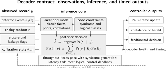
A decoder is a pipeline, not only an algorithm. Detector events, analog readout, erasure or leakage flags, and calibration data define an observation $y$. A likelihood model and the code constraints assign posterior weight to logical equivalence classes. The output is a frame or feedforward decision, often accompanied by confidence and health information, under a throughput and latency deadline.

Three noise-model levels

Decoder benchmarks commonly use three progressively richer models.

model	noisy elements	record seen by decoder	main use
code capacity	data errors only; checks perfect	one exact syndrome	algebra, asymptotic baselines
phenomenological	data and check outcomes fail by a prescribed rule	repeated noisy syndromes	spacetime decoding without a gate schedule
circuit level	preparation, gates, idles, measurement, reset, leakage, and correlations	the implemented circuit record	hardware and fault-tolerance claims

A threshold or runtime measured at one level cannot be transferred to another without qualification. Circuit-level faults can produce diagonal spacetime events, multi-detector correlations, hook errors, persistent leakage, and boundary effects absent from code-capacity noise.

Decoding Is Logical-Class Inference

Let $\mathcal S\subset\mathcal P_n$ be the stabilizer group of an $[[n,k,d]]$ code. A syndrome is a binary vector

$$s(E) \in \mathbb F_2^{n-k}$$

whose entries record whether a Pauli error $E$ commutes or anticommutes with the chosen stabilizer generators. Fix one Pauli $T_s$ with syndrome $s$. Every Pauli error with that syndrome can be written, up to phase, as

$$E = T_s L_\ell S, \qquad S\in\mathcal S,$$

where $L_\ell$ represents one of the $4^k$ logical Pauli classes in $N(\mathcal S)/\mathcal S$.

The syndrome fixes $T_s$ but does not reveal $\ell$. Multiplication by a stabilizer changes the microscopic representative without changing its action on the code space. Multiplication by a nontrivial logical Pauli preserves the syndrome but changes the encoded state. The decoder’s essential decision is therefore $\ell$, not the exact $E$.

If $y$ denotes the complete observed record and $\mathcal E_{s,\ell}$ is the set of physical fault histories compatible with syndrome $s$ and logical class $\ell$, then the Bayesian target is

$$\Pr(\ell\mid y) = \frac{1}{Z(y)} \sum_{E\in\mathcal E_{s,\ell}} \Pr(y\mid E)\Pr(E).$$

An ideal maximum-likelihood logical decoder chooses

$$\widehat\ell(y) = \underset{\ell}{\operatorname{argmax}}\, \Pr(\ell\mid y).$$

The sum is the mathematical expression of degeneracy. A decoder that chooses the single most likely physical error instead may select a different logical class from one that contains many individually less likely representatives.

Central distinction

A recovery succeeds when its product with the actual error is a stabilizer. Reconstructing the physical fault exactly is unnecessary, and can be the wrong optimization objective.

Hard and soft information

A hard decoder receives discrete outcomes such as syndrome bits. A soft decoder also receives reliability information:

$$y = \left( s,\, r,\, f_{\rm era},\, f_{\rm leak},\, \theta_{\rm cal} \right),$$

where $r$ may contain analog readout values, $f_{\rm era}$ known erasure locations, $f_{\rm leak}$ leakage indicators, and $\theta_{\rm cal}$ current calibration parameters. Thresholding $r$ before decoding is a lossy compression unless the thresholded bit is a sufficient statistic for the channel.

Soft information is especially valuable near a decision boundary. A weak measurement outcome, a GKP residue near the edge of a lattice cell, and a qubit flagged as leaked should not carry the same certainty as ordinary hard bits.

Worked Example: A Three-Qubit Repetition Code

Consider the bit-flip repetition code with checks

$$S_1=Z_1Z_2, \qquad S_2=Z_2Z_3,$$

and logical operator

$$\overline X=X_1X_2X_3.$$

Write syndrome bit $1$ when an error anticommutes with a check. The syndrome

$$s=(1,0)$$

is compatible with both

$$E_0=X_1$$

and

$$E_1=X_2X_3 = \overline X E_0.$$

The two explanations differ by a logical bit flip. If independent bit-flip probabilities are $p_1,p_2,p_3$, their exact probabilities are

$$\begin{aligned} \Pr(E_0) &= p_1(1-p_2)(1-p_3), \\ \Pr(E_1) &= (1-p_1)p_2p_3. \end{aligned}$$

The maximum-likelihood decision corrects with $X_1$ when the first quantity is larger and chooses the other logical class when the second is larger. For equal $p_i=p<1/2$, the weight-one explanation wins. That familiar minimum-weight rule is therefore a consequence of a particular prior, not a definition of decoding.

This example also shows why a decoder must know what its output means. Applying $X_1$ when the actual error was $X_2X_3$ leaves $\overline X$. Both candidate errors satisfy the measured checks.

From Circuit Records to Detector Models

Repeated extraction is usually expressed in terms of detectors: parities of measurement outcomes that are deterministic in a fault-free circuit. For a binary stabilizer outcome $m_a(t)$,

$$d_a(t) = m_a(t)\oplus m_a(t-1)$$

is a common bulk detector. Initial and final time boundaries require separate definitions based on preparation and terminal data measurements.

A detector error model describes elementary fault mechanisms $f_j$. Mechanism $j$ occurs with probability $p_j$, flips a detector set $D_j$, and may flip a logical-observable vector $\lambda_j$. A sampled fault set $F$ produces

$$\begin{aligned} d &= \bigoplus_{j\in F} \chi(D_j), \\ \ell &= \bigoplus_{j\in F} \lambda_j. \end{aligned}$$

Here $\chi(D_j)$ is the incidence vector of the affected detectors. This representation separates circuit simulation from classical inference, but it is still a model. If faults are assumed independent when the hardware produces bursts or persistent leakage, the posterior can be badly miscalibrated.

Graphlike and hypergraph mechanisms

If every modeled mechanism flips at most two detectors, each mechanism can be represented as an edge joining two detector vertices or one detector to a boundary. The decoding problem is then graphlike.

A single mechanism that flips three or more detectors is a hyperedge. Breaking that hyperedge into ordinary edges can lose correlations or introduce artificial explanations. Circuit-level $Y$ faults, leakage, crosstalk, and multi-qubit events are common reasons that a realistic detector model is not exactly graphlike.

Likelihood Weights

Suppose a candidate graph edge $e$ represents an independent Bernoulli fault with probability $p_e$. For a fault chain $F$,

$$\Pr(F) = \prod_{e\in F}p_e \prod_{e\notin F}(1-p_e).$$

Removing a candidate-independent constant from the negative log likelihood gives

$$-\log\Pr(F) = \sum_{e\in F} w_e +\text{constant},$$

with log-odds weight

$$w_e = \log \left( \frac{1-p_e}{p_e} \right).$$

Thus minimum total weight is maximum likelihood for the modeled fault configuration under the independence assumptions. Three cautions follow:

1. geometric length is a likelihood only when equal-length steps have the same probability;
2. minimum-weight configuration is not automatically maximum-likelihood logical class because class probabilities sum over degenerate paths;
3. negative weights can occur when $p_e>1/2$, signaling that the chosen reference event or graph representation should be reconsidered.

Major Decoder Families

No decoder dominates for every code and noise model.

family	natural structure	main strength	characteristic limitation
minimum-weight perfect matching	pair-created defects on a graph	mature, accurate, and highly optimized	graphlike approximation and incomplete degeneracy
union–find and clustering	local syndrome clusters and erasures	near-linear growth and hardware-friendly locality	heuristic choices can reduce accuracy
belief propagation	sparse Tanner graph with soft priors	parallel message passing and broad qLDPC applicability	loops, degeneracy, and trapping sets
tensor-network or renormalization	local graphical model	captures class sums and correlations systematically	approximation width and memory cost
local search and ordered statistics	sparse constraints plus reliability ranking	repairs message-passing failures	tunable combinatorial post-processing
learned decoder	representative labeled data	absorbs complex correlations and side information	training, drift, certification, and deployment cost

Minimum-weight perfect matching

Minimum-weight perfect matching, or MWPM, represents detection events as vertices and candidate pair connections as weighted edges. Boundaries are included as legal endpoints. A perfect matching pairs every event, possibly to a boundary, with minimum total weight. Paths associated with the matched pairs define a correction class.

MWPM is well matched to topological codes when sparse elementary faults create event pairs. It has several practical refinements:

• edge weights can come from a calibrated circuit-level detector model;
• time-like and diagonal edges represent measurement and propagated faults;
• boundary handling encodes preparation, readout, defects, and code deformation;
• correlated matching can partially couple $X$- and $Z$-type information;
• sparse implementations avoid constructing a dense all-pairs graph.

Matching does not, by itself, sum the probability of every degenerate path or represent arbitrary hyperedges. Its quality therefore depends on how faithfully the graph and weights compress the underlying channel.

Union–find and clustering

A union–find decoder begins with clusters around detection events. Clusters grow across low-cost edges and merge when they meet. Growth continues until each connected component has a syndrome parity compatible with a local correction or an allowed boundary. A peeling step on a spanning forest then constructs the correction.

The disjoint-set operations behind union–find have almost-linear worst-case complexity,

$$O\!\left(n\alpha(n)\right),$$

where $\alpha$ is the inverse Ackermann function and grows extremely slowly. The decoder is naturally local and handles known erasures well. Weighted growth, cluster scheduling, boundary policy, and circuit-level extensions matter in practice; the complexity bound alone does not establish a logical error rate or a hardware latency.

Belief propagation

Belief propagation, or BP, passes likelihood messages on a Tanner graph. For a binary parity system

$$He^{\mathsf T}=s,$$

let

$$L_i = \log \frac{\Pr(e_i=0)} {\Pr(e_i=1)}$$

be the prior log-likelihood ratio. A variable-to-check update is

$$L_{i\to a} = L_i + \sum_{b\in\mathcal N(i)\setminus a} L_{b\to i},$$

and a check-to-variable update is

$$\begin{aligned} L_{a\to i} = 2\,\operatorname{atanh} \bigg[ (-1)^{s_a} \prod_{j\in\mathcal N(a)\setminus i} \tanh\!\left( \frac{L_{j\to a}}{2} \right) \bigg]. \end{aligned}$$

On a tree, these updates recover exact local marginals after enough iterations. Quantum LDPC Tanner graphs contain cycles, often many short ones required by CSS orthogonality. Messages then become correlated; BP may oscillate, stop at an inconsistent word, or favor a poor representative of a degenerate class.

Common remedies include damping, randomized schedules, min-sum approximations, quaternary messages that retain $X$–$Z$ correlation, guided decimation, and learned message updates.

Belief propagation with ordered statistics

BP with ordered-statistics decoding, or BP+OSD, uses BP’s soft reliabilities to rank variables. It selects an information set, solves the syndrome constraint, and searches low-order changes among the least reliable decisions. The OSD stage often repairs a BP estimate that does not satisfy the syndrome or that lands in a poor local basin.

The search order is an accuracy–runtime parameter. Reporting only the name BP+OSD omits the iteration count, damping, OSD order, information-set rule, stopping condition, and runtime tail that define the implemented decoder.

Tensor-network and renormalization decoders

Maximum-likelihood logical decoding is a partition-function problem: sum the probability of all fault configurations in each logical class. Tensor-network decoders approximate those sums by contracting a graphical model with bounded bond dimension. Renormalization decoders coarse-grain local syndrome regions while passing effective probability distributions to larger scales.

These approaches can account for degeneracy and local correlations more directly than a single-path decoder. Their cost is controlled by contraction order, bond dimension, truncation, and geometry. A larger approximation parameter generally improves accuracy while increasing time and memory.

Local search, peeling, and erasure decoding

When the locations of errors are known but their Pauli values are not, as in an erasure channel, decoding is often much easier. Linear algebra, peeling, or cluster growth can determine whether the erased support contains a logical operator and construct a compatible correction.

For unknown errors, local search methods flip small sets of variables or checks that improve a score. Small-set-flip decoders exploit expansion in specific qLDPC constructions. Localized-statistics and beam-search methods retain or repair several candidate explanations. These methods are not interchangeable: a proof for one code family and adversarial error radius does not establish a stochastic circuit-level threshold for another.

Neural and learned decoders

A learned decoder represents a map such as

$$f_\theta(y) \longrightarrow \widehat{\Pr}_\theta(\ell\mid y),$$

where $\theta$ is fitted from simulated or experimental records. Convolutional networks exploit spatial locality; recurrent and transformer models process long syndrome histories; graph neural networks can follow irregular check connectivity; learned message passing inserts trainable updates into a structured decoder.

Learned methods can absorb correlations, leakage indicators, analog readout, and calibration features that are awkward to encode by hand. They also create specific obligations:

• training labels must correspond to the intended logical task;
• training, validation, and test shots must be separated;
• performance must be checked across code sizes and round counts;
• synthetic pretraining and experimental fine-tuning must be distinguished;
• drift and out-of-distribution faults need detection and fallback behavior;
• inference latency, accelerator transfer, memory, and power must be counted;
• a higher offline accuracy does not prove real-time deployability.

A neural decoder is therefore neither intrinsically superior nor intrinsically untrustworthy. It is an estimator whose information, data distribution, architecture, and operating envelope must be reported.

Match the Decoder to the Channel

Independent CSS decoding can discard Pauli correlations

CSS Codes owns the split syndrome equations and logical quotient criterion. This page retains joint priors, correlations, degeneracy-aware posterior inference, algorithms, confidence, throughput, and latency.

For a CSS code, it is convenient to decode $X$ and $Z$ components separately. That is exact only when the prior factorizes appropriately. A physical $Y$ fault contributes both components. Separate decoders can count it as two independent events and assign the wrong likelihood.

Joint quaternary BP, correlated matching, tensor-network models, or a post-processing stage can retain some of this information. Whether the gain is worth the computational cost depends on the measured $X$–$Y$–$Z$ channel.

Bias changes weights and sometimes geometry

If dephasing is much more likely than bit flipping, equal graph weights waste known information. A tailored decoder changes likelihoods; a tailored code can also change check geometry so that the dominant faults require longer logical paths. Decoder and code adaptation must be evaluated together.

Erasure flags are information, not errors

An erasure location says where a fault occurred without necessarily revealing its Pauli action. This side information can turn a hard search over all qubits into a constrained solve on the erased support. A false erasure flag and a missed erasure have different consequences, so flag fidelity belongs in the channel model.

Analog syndromes should remain analog when useful

The GKP Codes page derives lattice-residue likelihoods. Similar reasoning applies to continuous readout voltages from discrete-variable checks. The outer decoder can use a log-likelihood ratio instead of a thresholded sign:

$$\Lambda(r) = \log \frac{p(r\mid s=0)} {p(r\mid s=1)}.$$

Analog information helps only when the likelihood model is calibrated. A mis-scaled confidence can overweight a bad measurement more severely than a hard decision would.

Leakage creates memory

A leaked qubit can corrupt several later gates and syndrome rounds. Modeling each affected detector as an independent Pauli event misses the shared hidden cause. Useful responses include leakage-reduction units, hidden-state models, longer detector edges or hyperedges, leakage-aware weights, erasure conversion, and controller actions that remove or replace the leaked carrier.

Coherent noise is not a Pauli sample by default

Syndrome measurement often converts part of a coherent error into a classical mixture, but repeated coherent faults can interfere and produce logical behavior not captured by an independently sampled Pauli model. Pauli twirling is a modeling approximation unless randomized compiling or another physical mechanism implements it operationally. Decoder performance under a Pauli surrogate must not be presented as a theorem about the original coherent channel.

Pauli Noise and Depolarizing Channels owns the physical-Pauli to syndrome and logical-class probability pushforward and the correlated-versus-independent audit; this page retains decoder priors, logical-class inference algorithms, likelihood models, real-time constraints, and decoder evaluation.

Model Learning and Correlated Noise

The decoder prior should be informed by the same circuit context in which it will operate. Detector correlations can estimate elementary fault probabilities:

$$C_{ab} = \langle d_a d_b\rangle -\langle d_a\rangle\langle d_b\rangle.$$

Pair correlations can calibrate graph edges, but they do not uniquely identify all higher-order mechanisms. A burst that flips many detectors, two simultaneous pair faults, and a persistent hidden leakage state can produce similar low-order statistics.

A trustworthy calibration workflow therefore:

1. collects timestamped records under the actual extraction schedule;
2. keeps analog and flag information until its value has been assessed;
3. fits a model with explicit spatial and temporal support;
4. validates predicted detector and logical statistics on held-out data;
5. monitors drift and changes model versions deliberately;
6. tests rare-event and adversarial perturbations;
7. records the fallback used when confidence or system health is poor.

More expressive models are not automatically better. A highly parameterized model can overfit a finite calibration set, increase update latency, or assign confident probabilities to unseen faults.

Real-Time Decoding

Throughput and latency are different

Suppose $N_{\rm det}$ detector records, each represented by $b_{\rm rec}$ bits or bytes, arrive every cycle of duration $\tau_{\rm cyc}$. The raw input bandwidth is

$$B_{\rm in} = \frac{N_{\rm det}b_{\rm rec}} {\tau_{\rm cyc}}.$$

Let $\lambda$ be the long-run work-arrival rate and $\mu$ the decoder service rate in matching units. Avoiding an ever-growing backlog requires

$$\mu>\lambda.$$

That condition is necessary but not sufficient. Bursts and runtime variation can violate a control deadline even when the mean service rate is adequate. The operational requirement is a tail probability,

$$\Pr \left( T_{\rm end\mbox{-}to\mbox{-}end} > T_{\rm deadline} \right) \leq \epsilon_{\rm late}.$$

End-to-end time includes acquisition, classification, transport, decoding, frame reconciliation, decision distribution, and actuation. Quoting only kernel runtime excludes the parts most likely to differ between a workstation benchmark and a deployed controller.

Streaming and windowed decoding

An unbounded syndrome history cannot be re-decoded from scratch after every round. Streaming decoders process new data incrementally. Windowed decoders split spacetime into overlapping blocks, commit corrections in an interior region, and reconcile uncertain boundaries with later windows.

The overlap must be wide enough that likely fault chains do not get cut into inconsistent decisions. Parallel windows can raise throughput, but they add boundary messages, buffers, scheduling, and failure modes. A window scheme should report its logical-accuracy penalty and heralded-failure rate as well as speed.

A Pauli frame buys time, not unlimited time

Most inferred Pauli corrections need not be applied physically. They can be tracked in a Pauli frame and propagated through later Clifford operations. This removes a per-cycle physical-correction deadline.

Hard deadlines remain at:

• adaptive measurements;
• non-Clifford gate injection and feedforward;
• code deformation and lattice surgery;
• qubit reuse and reset;
• leakage response;
• terminal logical interpretation;
• branch-dependent scheduling.

A decoder that keeps up on average but misses those boundaries can still stall or corrupt the logical computation.

Classical fault tolerance matters

The decoder hardware can itself drop records, suffer memory errors, miss deadlines, or become unavailable. Large systems need checksums, redundant links, bounded queues, health monitoring, deterministic failure policies, and possibly replicated decoding. Classical redundancy is part of the fault-tolerant architecture, not an external assumption.

How Decoder Claims Should Be Evaluated

Accuracy metrics

Useful accuracy quantities include:

• logical failure probability per round or per logical operation;
• logical channel or basis-resolved failure rates;
• suppression factor when distance increases under a fixed contract;
• threshold for a declared code family and noise model;
• comparison with exact decoding at small sizes;
• calibration and confidence reliability;
• heralded-failure and postselection rates.

A pseudothreshold at one finite distance is not an asymptotic threshold. The Threshold Theorem separates proof bounds, crossings, pseudothresholds, and device evidence. A memory decoder’s logical error per cycle is not an encoded-gate error rate.

Systems metrics

Useful systems quantities include:

• sustained rounds or detector events per second;
• mean, median, high-quantile, and worst observed latency;
• queue depth and memory footprint;
• host-to-accelerator and controller transport;
• parallelism and number of cores or accelerators;
• power, area, and cryogenic boundary when relevant;
• preprocessing, model-loading, and calibration cost;
• behavior under bursts, missing records, and model updates.

Fair comparison checklist

Two decoder curves are comparable only if they use the same:

1. code family, distance, boundaries, and logical observable;
2. extraction circuit and number of rounds;
3. physical noise model and parameters;
4. analog, erasure, leakage, and calibration information;
5. treatment of initialization and final measurement;
6. acceptance and heralding policy;
7. runtime hardware and implementation language;
8. logical-error estimator and uncertainty method.

An oracle decoder given the exact sampled fault locations is a bound, not a deployable baseline. Likewise, an offline decoder may be an accuracy reference without satisfying the online control contract.

Evidence Through August 2026

The major decoder families are established algorithms, but no universal winner is established.

• Sparse-blossom simulations published in 2025 processed both bases of a distance-17 surface-code circuit with $0.1\%$ circuit-level depolarizing noise in less than one microsecond per round on one specified CPU core. This is strong implementation evidence for graphlike matching, not an integrated processor benchmark for arbitrary noise.
• A 2025 superconducting experiment integrated streaming decoding with a distance-5 surface-code memory. It maintained below-threshold performance for runs up to one million cycles and reported a roughly constant $63\pm17\,\mu{\rm s}$ average terminal decoder latency while processing a $1.1\,\mu{\rm s}$ syndrome cycle. Throughput and reaction latency were deliberately distinct.
• Hardware studies in 2025 demonstrated megahertz collision-clustering decoding in FPGA and ASIC implementations for simulated surface-code workloads. They establish resource and throughput evidence for that model, not end-to-end logical performance on live qubits.
• The AlphaQubit work published in 2024 improved decoding accuracy on experimental distance-3 and distance-5 surface-code data and on simulated systems through distance 11 using a recurrent transformer with soft and leakage information. Its reported high-accuracy mode was an offline decoder, so accuracy does not by itself establish a control-loop deadline.
• A 2026 experiment inferred decoder weights from syndrome correlations in a distance-3 surface-code circuit and observed correlated detector patterns extending over several cycles, plausibly associated with leakage. This supports circuit-context calibration while also showing why an independent edge model can be incomplete.

These results demonstrate fast, learned, calibrated, and integrated decoding in bounded regimes. They do not establish that one algorithm simultaneously maximizes accuracy, handles every relevant correlation, scales to a useful fault-tolerant workload, and meets all latency, power, and reliability constraints.

Practical Decoder Workflow

For a new code or device:

1. define logical observables, detector conventions, and time boundaries;
2. derive a detector or factor-graph model from the actual extraction circuit;
3. identify available hard, analog, erasure, and leakage information;
4. establish an exact or high-accuracy small-instance reference;
5. choose at least one fast baseline matched to the graph structure;
6. calibrate priors on training data and freeze a test set;
7. sweep code size, physical error rate, rounds, and drift conditions;
8. report logical accuracy together with runtime and resource distributions;
9. test streaming boundaries, missing data, bursts, and fallback behavior;
10. version the model, decoder, calibration, and controller together.

This workflow prevents an algorithmic improvement from being confused with a change in information, simulator, or benchmark.

Common Mistakes

Treating the syndrome as an error location

The syndrome gives constraints or endpoints. It does not generally identify a unique fault path.

Correcting the most likely error instead of the most likely class

Quantum degeneracy requires summing probabilities over stabilizer-equivalent representatives. A single-path approximation can be useful, but its objective should be named.

Using geometric distance as a universal weight

Distance is a proxy for negative log likelihood only under a sufficiently uniform, independent model. Hardware asymmetry and circuit propagation change the weights.

Quoting a decoder threshold without the contract

Thresholds belong to a code family, syndrome circuit, noise model, decoder, and metric. They are not intrinsic constants of algorithm names.

Comparing hard and soft decoders as if they saw the same input

Extra analog, erasure, or leakage information can improve any suitable inference method. The information advantage must be separated from the algorithm advantage.

Equating simulated kernel speed with real-time operation

A fast inner loop may omit transport, buffering, final-boundary processing, and feedforward. Real time is an end-to-end systems property.

Reporting only mean latency

Rare latency spikes can violate a logical deadline or accumulate a queue. High-quantile and failure behavior matter.

Training and testing a learned decoder on the same distribution slice

Randomly splitting strongly correlated shots, tuning on the test set, or using simulator labels unavailable in hardware can produce optimistic results.

Ignoring drift and rare correlated faults

A decoder fitted to average pair correlations can miss bursts, leakage, or context-dependent faults that dominate the logical tail.

Physically applying every Pauli correction

A Pauli-frame update is usually safer and cheaper. Physical action is needed only where the control protocol requires it.

Connections

• Logical Benchmarking defines held-out logical accuracy, suppression, break-even, acceptance, latency-mode, and clustered-statistics tests for delivered decoder behavior.
• Stabilizer Formalism supplies the quotient structure that makes logical-class decoding precise.
• Color Codes owns the three-colored face-check geometry and the projection/restriction-plus-lifting interface; this page retains general inference, calibration, confidence, throughput, and latency.
• Surface Code gives the canonical spacetime-graph example.
• Quantum LDPC Codes develops sparse-check families, BP+OSD use, and construction-specific provable decoders.
• GKP Codes derives analog lattice likelihoods for a bosonic inner code.
• Control, Readout, and Calibration owns acquisition, controller, and calibration hardware.
• Reporting Standards owns reproducible metric, uncertainty, and disclosure conventions.

Exercises

1. Recovery classes

Let $E$ and $E'$ have the same stabilizer syndrome. Show that $E'E^\dagger\in N(\mathcal S)$. Explain why $E$ and $E'$ are equivalent recoveries exactly when this product lies in $\mathcal S$ up to phase.

Solution

For every stabilizer generator $g$, equal syndromes mean that $E$ and $E'$ have the same commutation sign with $g$. Moving $g$ through $E'E^\dagger$ therefore produces the product of two equal signs, which is $+1$. Hence

$$[E'E^\dagger,g]=0$$

for every $g\in\mathcal S$, so

$$E'E^\dagger\in N(\mathcal S).$$

If the product is a stabilizer, the two errors act identically on the code space. If it is in $N(\mathcal S)\setminus\mathcal S$, it acts as a nontrivial logical Pauli, so choosing one correction for the other causes a logical failure.

2. Nonuniform repetition-code priors

For the syndrome $(1,0)$ in the worked example, derive the condition under which $X_2X_3$ is more likely than $X_1$. Evaluate it for $p_1=10^{-3}$ and $p_2=p_3=0.1$.

Solution

Choose $X_2X_3$ when

$$(1-p_1)p_2p_3 > p_1(1-p_2)(1-p_3).$$

For the stated values,

$$\begin{aligned} \Pr(X_2X_3) &= 0.999(0.1)^2 = 9.99\times10^{-3}, \\ \Pr(X_1) &= 10^{-3}(0.9)^2 = 8.1\times10^{-4}. \end{aligned}$$

The weight-two explanation is more than an order of magnitude likelier because qubit 1 is much cleaner. Minimum Hamming weight would make the wrong Bayesian choice.

3. Matching weights

Starting from independent edge probabilities, derive $w_e=\log[(1-p_e)/p_e]$. For $p_a=10^{-2}$ and $p_b=10^{-3}$, compare the weight of one $a$ edge with two $b$ edges.

Solution

For a candidate set $F$,

$$\Pr(F) = \prod_{e\in F}p_e \prod_{e\notin F}(1-p_e).$$

Factoring out $\prod_e(1-p_e)$ gives

$$\Pr(F) \propto \prod_{e\in F} \frac{p_e}{1-p_e}.$$

Taking minus the logarithm yields the stated additive weight. Numerically,

$$w_a = \log 99 \approx 4.60,$$

while

$$2w_b = 2\log 999 \approx 13.81.$$

Under this model, one $a$ edge is much more likely than two $b$ edges even if the geometric alternatives have lengths one and two.

4. Most-likely representative versus class

Suppose logical class $A$ contains one compatible error of probability $0.30$, while class $B$ contains four compatible errors of probability $0.10$ each. What do maximum-a-posteriori physical-error decoding and maximum-likelihood logical-class decoding choose?

Solution

The most likely individual error has probability $0.30$, so physical-error MAP chooses class $A$. The class probabilities are

$$\Pr(A\mid y)=0.30, \qquad \Pr(B\mid y)=0.40,$$

up to their common normalization. Logical-class maximum likelihood chooses $B$. The example isolates the role of degeneracy.

5. One belief-propagation check

A parity check has syndrome $s_a=0$ and receives two incoming variable messages $L_{1\to a}=L_{2\to a}=2$. Compute the outgoing message to a third variable.

Solution

The update is

$$L_{a\to3} = 2\,\operatorname{atanh} \left[ \tanh^2(1) \right].$$

Since $\tanh(1)\approx0.7616$,

$$L_{a\to3} \approx 2\,\operatorname{atanh}(0.5800) \approx 1.33.$$

The positive sign favors $e_3=0$, consistent with an even-parity check whose other two variables are each more likely to be zero.

6. Throughput and deadline

A device emits $2\times10^5$ detector bits every $2\,\mu{\rm s}$. Find the raw bit rate. A decoder sustains $1.2\times10^{11}$ bits per second but has a $99.999$th-percentile end-to-end latency above an adaptive deadline. Which real-time condition passes and which fails?

Solution

The input rate is

$$B_{\rm in} = \frac{2\times10^5} {2\times10^{-6}\ {\rm s}} = 10^{11}\ {\rm bit\,s^{-1}}.$$

The sustained service rate is $20\%$ higher, so the mean-throughput stability condition passes. The latency-tail condition fails because some required decisions arrive after the adaptive deadline. Both conditions are necessary for that workload.

7. A correlated Pauli prior

A qubit has

$$\Pr(I)=0.97, \quad \Pr(X)=0.01, \quad \Pr(Y)=0.015, \quad \Pr(Z)=0.005.$$

Compare the true probability that both binary components are present with the product obtained by treating $X$ and $Z$ components independently.

Solution

Both components are present exactly for a $Y$ fault, so

$$\Pr(x=1,z=1)=0.015.$$

The marginal component probabilities are

$$\Pr(x=1)=\Pr(X)+\Pr(Y)=0.025$$

and

$$\Pr(z=1)=\Pr(Z)+\Pr(Y)=0.020.$$

An independent model assigns

$$\Pr(x=1)\Pr(z=1) = 5\times10^{-4},$$

underestimating the joint event by a factor of $30$. Separate CSS decoding can therefore discard substantial information.

8. Design a decoder benchmark

Specify a minimal benchmark that fairly compares a matching decoder with a learned decoder for a repeated surface-code memory.

Solution

A defensible benchmark fixes the code distances and boundaries, extraction circuit, number of rounds, physical or empirical noise model, initialization, terminal measurement, and logical observable. Both decoders receive the same hard or soft record. Training shots are separated from validation and test shots, and the matching weights are calibrated without test leakage.

Report logical failure with confidence intervals, distance scaling, and performance under a held-out drift or burst set. On the same declared hardware, report sustained throughput, latency quantiles, memory, preprocessing, transport, and any accelerator cost. State whether each decoder is batch, streaming, or offline and whether either can herald or reject a run.

References

1. D. Gottesman, “Stabilizer codes and quantum error correction,” PhD thesis, California Institute of Technology (1997), arXiv:quant-ph/9705052.
2. E. Dennis, A. Kitaev, A. Landahl, and J. Preskill, “Topological quantum memory,” Journal of Mathematical Physics 43, 4452–4505 (2002), doi:10.1063/1.1499754.
3. J. Edmonds, “Paths, trees, and flowers,” Canadian Journal of Mathematics 17, 449–467 (1965), doi:10.4153/CJM-1965-045-4.
4. A. G. Fowler, A. C. Whiteside, and L. C. L. Hollenberg, “Towards practical classical processing for the surface code,” Physical Review Letters 108, 180501 (2012), doi:10.1103/PhysRevLett.108.180501.
5. S. Bravyi, M. Suchara, and A. Vargo, “Efficient algorithms for maximum likelihood decoding in the surface code,” Physical Review A 90, 032326 (2014), doi:10.1103/PhysRevA.90.032326.
6. G. Duclos-Cianci and D. Poulin, “Fast decoders for topological quantum codes,” Physical Review Letters 104, 050504 (2010), doi:10.1103/PhysRevLett.104.050504.
7. N. Delfosse and N. H. Nickerson, “Almost-linear time decoding algorithm for topological codes,” Quantum 5, 595 (2021), doi:10.22331/q-2021-12-02-595.
8. O. Higgott, “PyMatching: a Python package for decoding quantum codes with minimum-weight perfect matching,” ACM Transactions on Quantum Computing 3, article 16 (2022), doi:10.1145/3505637.
9. O. Higgott and C. Gidney, “Sparse blossom: correcting a million errors per core second with minimum-weight matching,” Quantum 9, 1600 (2025), doi:10.22331/q-2025-01-20-1600.
10. D. Poulin and Y. Chung, “On the iterative decoding of sparse quantum codes,” Quantum Information and Computation 8, 987–1000 (2008), doi:10.26421/QIC8.10-8, arXiv:0801.1241.
11. J. Roffe, D. R. White, S. Burton, and E. Campbell, “Decoding across the quantum low-density parity-check code landscape,” Physical Review Research 2, 043423 (2020), doi:10.1103/PhysRevResearch.2.043423.
12. C. Piveteau and J. M. Renes, “Quantum message-passing algorithm for optimal and efficient decoding,” Quantum 6, 784 (2022), doi:10.22331/q-2022-08-23-784.
13. C. T. Chubb and S. T. Flammia, “Statistical mechanical models for quantum codes with correlated noise,” Annales de l’Institut Henri Poincaré D 8, 269–321 (2021), doi:10.4171/AIHPD/105.
14. A. S. Darmawan and D. Poulin, “Tensor-network simulations of the surface code under realistic noise,” Physical Review Letters 119, 040502 (2017), doi:10.1103/PhysRevLett.119.040502.
15. G. Torlai and R. G. Melko, “Neural decoder for topological codes,” Physical Review Letters 119, 030501 (2017), doi:10.1103/PhysRevLett.119.030501.
16. J. Bausch et al., “Learning high-accuracy error decoding for quantum processors,” Nature 635, 834–840 (2024), doi:10.1038/s41586-024-08148-8.
17. X. Tan, F. Zhang, R. Chao, Y. Shi, and J. Chen, “Scalable surface-code decoders with parallelization in time,” PRX Quantum 4, 040344 (2023), doi:10.1103/PRXQuantum.4.040344.
18. Google Quantum AI and Collaborators, “Quantum error correction below the surface code threshold,” Nature 638, 920–926 (2025), doi:10.1038/s41586-024-08449-y.
19. B. Barber et al., “A real-time, scalable, fast and resource-efficient decoder for a quantum computer,” Nature Electronics 8, 84–91 (2025), doi:10.1038/s41928-024-01319-5.
20. A. Remm et al., “Experimentally informed decoding of stabilizer codes based on syndrome correlations,” Physical Review Research 8, 013044 (2026), doi:10.1103/z1ng-wg3k.