Magic State Distillation

A magic state is a nonstabilizer ancillary state whose consumption lets an otherwise stabilizer-based fault-tolerant architecture implement a non-Clifford operation. Magic state distillation is a postselected error-detection procedure: it consumes several imperfect resource states, uses protected stabilizer operations to test collective parity constraints, and conditionally returns fewer states with lower error.

This construction resolves a common architectural mismatch. Clifford gates, Pauli measurements, stabilizer preparations, and classical feedforward are often comparatively natural at the logical level, but they are not universal. A non-Clifford gate such as $T$ completes a universal set, yet implementing it directly and fault tolerantly can be expensive. The architecture therefore moves much of that difficulty offline: prepare noisy nonstabilizer states, purify them in factories, route accepted outputs to the data region, and consume them through a small injection gadget.

The word distillation can hide the engineering burden. A factory has a rejection probability, a finite output rate, logical faults in its Clifford circuit, routing and storage errors, decoder latency, and possibly correlated outputs. The useful question is not merely whether an ideal recurrence sends $p$ to $O(p^3)$. It is whether the complete factory supplies enough verified states, at the required logical error, when and where the algorithm needs them.

Canonical Scope

Stabilizer Formalism owns stabilizer states, logical Paulis, syndromes, and Clifford propagation. Universal Gate Sets owns universality and compilation into Clifford+$T$ or other logical alphabets. Fault-Tolerant Gates owns the general gadget contract, including error containment and teleportation-based gates. Resource Estimation owns the end-to-end cost model that combines state quality, acceptance, throughput, footprint, buffering, and compiled demand.

This page is the canonical home for $T$-state injection, noisy-state models, distillation maps, the 15-to-1 Reed–Muller protocol, recursive purification, protocol-family comparisons, and logical factory design. Surface-code patch operations belong with Surface Code, while Lattice Surgery owns protected patch-parity schedules and the routing and injection interfaces that connect factories to data blocks. Dated integrated-system claims belong with the Fault-Tolerant Quantum Computing Frontier.

Experimental statements below use an evidence cutoff of 11 August 2026. The mathematical principles of injection and distillation are established. The scale, throughput, and integrated reliability of practical factories remain architecture-dependent research questions.

Quantum Error Correction and Fault Tolerance routes here when universal completion requires a non-stabilizer resource and a factory ledger; this page retains state injection, distillation maps, protocol families, correlated-input limits, factory throughput, backpressure, failure, and evidence.

Magic Relative to Stabilizer Operations

For a single qubit, define

$$T = \begin{pmatrix} 1&0\\ 0&e^{i\pi/4} \end{pmatrix}, \qquad S=T^2,$$

and the associated resource state

$$|T\rangle =T|+\rangle = \frac{|0\rangle+e^{i\pi/4}|1\rangle}{\sqrt 2}.$$

The Clifford group normalizes the Pauli group. Stabilizer states processed by Clifford unitaries, Pauli measurements, and classical feedforward remain inside the stabilizer framework, which admits efficient classical simulation under the usual Gottesman–Knill assumptions. The state $|T\rangle$ lies outside the stabilizer polytope. Supplying it permits a Clifford circuit to implement $T$, so it is a resource for universality in that restricted operational theory.

Magic is therefore relative to an allowed free-operation set. The same physical operation can be cheap in one code and expensive in another. A code with a transversal $T$ gate may instead pay for difficult Clifford gates, code switching, nonlocal checks, or a more demanding decoder. Saying that ”$T$ gates are expensive” is shorthand for a common architecture-level cost model, not a theorem about the abstract unitary $T$.

Other resource bases are possible. One can distill eigenstates of Hadamard, prepare three-qubit $CCZ$ states, inject arbitrary-angle rotations, or switch to a code where a desired gate is native. The correct resource is the one matched to the compiled gate set and the fault-tolerant substrate.

Exact T-State Injection

Let the data qubit be

$$|\psi\rangle=a|0\rangle+b|1\rangle,$$

and prepare an ancillary $|T\rangle$. Apply CNOT with the data as control and the ancilla as target. The joint state becomes

$$\frac{1}{\sqrt 2} \left[ a|0\rangle\bigl(|0\rangle+e^{i\pi/4}|1\rangle\bigr) + b|1\rangle\bigl(|1\rangle+e^{i\pi/4}|0\rangle\bigr) \right].$$

Measure the ancilla in the computational basis. For outcome $m=0$, the unnormalized data state is

$$\frac{1}{\sqrt 2} \left(a|0\rangle+e^{i\pi/4}b|1\rangle\right) = \frac{1}{\sqrt 2}T|\psi\rangle.$$

For outcome $m=1$, it is

$$\frac{1}{\sqrt 2} \left(e^{i\pi/4}a|0\rangle+b|1\rangle\right) = \frac{e^{i\pi/4}}{\sqrt 2}T^\dagger|\psi\rangle.$$

Each outcome has probability $1/2$ in the ideal circuit. Since

$$S T^\dagger=T,$$

an $S$ correction for $m=1$ makes both branches implement $T$, up to a global phase. In a fault-tolerant implementation, the correction is often tracked in a Clifford frame rather than immediately enacted.

This identity explains why a verified ancillary state can replace a direct logical $T$ gate, but it does not by itself prove fault tolerance. The CNOT, measurement, feedforward, ancilla transport, and frame update must satisfy the same containment requirements as any other fault-tolerant gate gadget. A bad resource state can also place a logical error directly on the data. Factory output quality is therefore part of the algorithm’s logical error budget.

A Noisy T-State Model

An arbitrary one-qubit preparation error need not be diagonal in the $\{|T\rangle,Z|T\rangle\}$ basis. Define

$$W = \frac{X+Y}{\sqrt 2} = e^{-i\pi/4}SX.$$

This is a Hermitian Clifford unitary. Its eigenstates are

$$W|T\rangle=|T\rangle, \qquad W|T_\perp\rangle=-|T_\perp\rangle, \qquad |T_\perp\rangle=Z|T\rangle.$$

Randomly applying $I$ or $W$ and forgetting the choice implements the twirl

$$\mathcal T_W(\rho) = \frac{1}{2}\left(\rho+W\rho W\right) = (1-p)|T\rangle\!\langle T| +p|T_\perp\rangle\!\langle T_\perp|,$$

where

$$p=\langle T_\perp|\rho|T_\perp\rangle.$$

The diagonal model turns preparation noise into a classical $Z$-error variable before an ideal $T$ state. It is convenient for deriving exact distillation polynomials. It is not automatically a faithful description of a factory. One-copy twirling removes local coherence, but it does not erase correlations among different inputs, leakage outside the qubit subspace, time-dependent drift, or faults in the twirl itself. Deliberately randomizing Pauli or Clifford frames can make a stochastic model more appropriate, but the claimed noise reduction must be justified for the implemented protocol.

The scalar $p$ is also not the only possible quality metric. Depending on the use case, one may need state fidelity, trace distance, diamond-norm error of the injected channel, leakage probability, or a composable bound conditioned on acceptance. A reported fidelity without the acceptance event and its conditioning can be misleading.

Distillation as a Conditional Channel

An $n$-to-$k$ protocol is a trace-nonincreasing channel $\mathcal D_{\rm acc}$ for the accepted syndrome outcomes. Given an input state $\rho_n$, its acceptance probability and conditional output are

$$P_{\rm acc}(\rho_n) = \operatorname{Tr}\mathcal D_{\rm acc}(\rho_n),$$ $$\rho_{k,\rm out} = \frac{\mathcal D_{\rm acc}(\rho_n)} {P_{\rm acc}(\rho_n)}.$$

The rejected branch is discarded or recycled only if a separate argument shows that recycling is valid. Postselection does not make the rejection cost disappear.

For independent diagonal inputs of error $p$, many protocols reduce to a one-dimensional map

$$p_{\rm out}=f(p), \qquad P_{\rm acc}=A(p).$$

If

$$f(p)=C p^r+O(p^{r+1}), \qquad r>1,$$

then the protocol suppresses sufficiently small input error to order $r$. The coefficient $C$ can matter as much as the order at practical error rates. A protocol threshold is a nonzero fixed point $p_*$ for which $f(p)<p$ below the relevant branch. It assumes the protocol’s specified input model and ideal stabilizer operations. It is neither a hardware error-correction threshold nor a universal boundary for distillable magic.

The expected raw-state cost per accepted output for one idealized stage is

$$C_1 = \frac{n}{kP_{\rm acc}}.$$

This number omits logical qubits, code cycles, storage, routing, classical latency, and the burstiness caused by rejection. It is a yield metric, not a complete resource estimate.

The 15-to-1 Reed–Muller Protocol

The canonical $T$-state protocol descends from the punctured quantum Reed–Muller $[[15,1,3]]$ code. In a circuit-level description, fifteen noisy resource states provide non-Clifford rotations to a Clifford encoding and checking network. Four independent $X$-type parity checks detect the lowest weight input-error patterns. The run is accepted only when all check outcomes are trivial; Clifford decoding then produces one candidate output.

Equivalent circuits may reverse $T$ and $T^\dagger$, conjugate checks, or absorb Clifford corrections into frames. Those convention changes do not alter the ideal input-output polynomial when $p$ denotes error in the matched magic-state basis.

Exact acceptance and output error

For fifteen independent twirled inputs, define

$$x=1-2p.$$

The exact ideal acceptance probability is

$$P_{\rm acc}(p) = \frac{1+15x^8}{16}.$$

The conditional output error is

$$p_{\rm out}(p) = \frac{ 1-15x^7+15x^8-x^{15} } {2\left(1+15x^8\right)}.$$

Expanding near $p=0$ gives

$$P_{\rm acc}(p) = 1-15p+105p^2-420p^3+O(p^4),$$ $$p_{\rm out}(p) = 35p^3+O(p^4).$$

All one- and two-input $Z$ errors are rejected. There are $35$ accepted weight-three patterns that act as a logical error, which gives the leading coefficient. The distance-three label alone predicts cubic suppression only after conditioning and only for the specified independent input model; the weight enumerator supplies the coefficient and the exact behavior away from $p=0$.

The nonzero useful fixed point is approximately

$$p_*=0.1414802927.$$

Below this value, the ideal map improves the state. Calling $14.1\%$ a “threshold” without the qualifier 15-to-1 protocol threshold under perfect Clifford operations and independent diagonal inputs invites the wrong comparison with physical gate thresholds.

A numerical example

For $p=10^{-3}$, the exact formulas give

$$P_{\rm acc} \approx 0.9851045810, \qquad p_{\rm out} \approx 3.51054\times10^{-8}.$$

The expected number of raw states per accepted output is therefore

$$\frac{15}{P_{\rm acc}} \approx 15.2268.$$

At $p=10^{-2}$, acceptance falls to about $0.86009$ and the output error is about $3.61\times10^{-5}$. At $p=0.1$, acceptance is only about $0.21979$ and the output error is about $0.04773$. The cubic asymptote is informative near zero, but the exact conditional map is the appropriate tool near the protocol threshold.

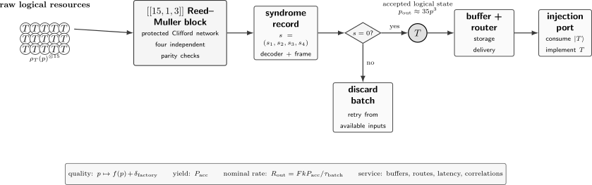
An idealized 15-to-1 factory. The polynomial $p_{\rm out}\approx35p^3$ and acceptance $P_{\rm acc}$ describe the independent-input, perfect-Clifford model. A complete factory must also account for logical circuit faults, correlations, buffering, routing, and decoder latency.

Recursive Distillation and Error Floors

One stage may not reach an algorithm’s target error. If accepted outputs from level $\ell-1$ become inputs to level $\ell$, an ideal recursive model gives

$$p_\ell=f_\ell(p_{\ell-1}).$$

For two 15-to-1 levels and $p_0=10^{-3}$, the leading-order recurrence gives

$$p_1\approx35p_0^3=3.5\times10^{-8},$$ $$p_2 \approx35p_1^3 \approx1.50\times10^{-21}.$$

The second number should trigger skepticism, not celebration. It assumes that every encoded Clifford operation, check measurement, reset, route, storage interval, and classical decision is perfect. A more useful stage model is

$$p_\ell \lesssim f_\ell(p_{\ell-1})+\delta_\ell,$$

where $\delta_\ell$ collects faults introduced by that protected factory level, including false acceptance. Once $f_\ell(p_{\ell-1})$ is below $\delta_\ell$, another ideal distillation round does not buy the advertised orders of magnitude. The code distance or verification strength at later levels may need to increase.

For stages with $n_\ell$ inputs and $k_\ell$ accepted outputs, the ideal expected raw-state cost obeys

$$C_\ell = C_{\ell-1} \frac{n_\ell}{k_\ell P_{{\rm acc},\ell}},$$

and hence

$$C_L = \prod_{\ell=1}^{L} \frac{n_\ell}{k_\ell P_{{\rm acc},\ell}}.$$

The product assumes that rejected batches can be retried independently and that upstream supply is available when needed. A real multilevel factory is a queueing network. A rejected high-level batch consumes accepted lower-level states that cannot be recovered, and finite buffers couple the stages.

Protocol Families

There is no universally best distillation code. The useful comparison axes are input-state type, output count, suppression order, threshold, acceptance, logical circuit depth, qubit footprint, connectivity, and sensitivity to correlated or biased noise.

Family	Resource and strategy	Main tradeoff
Bravyi–Kitaev 15-to-1	One $T$-type output from the punctured Reed–Muller code	Simple canonical cubic protocol; low output rate per block
Meier–Eastin–Knill 10-to-2	Two Hadamard-type outputs using error-detecting code gadgets	Better small-block yield in some regimes; quadratic suppression and a different resource basis
Bravyi–Haah triorthogonal blocks	Many $T$ outputs from matrices admitting transversal phase structure	Higher rate and tunable block size; more involved circuits and correlated-output analysis
Multilevel protocols	Couple several code levels so checks themselves use lower-quality resources	Improved asymptotic scaling; scheduling and fault accounting become less transparent
Synthillation	Combine synthesis of a multiqubit diagonal gate with purification	Can reduce cost for structured rotations; not interchangeable with a generic stream of $T$ states
$CCZ$ and Toffoli factories	Produce a three-qubit non-Clifford resource directly	Attractive when the workload consumes many Toffoli-like gates; output and catalyst correlations matter
Asymptotic constructions	Use growing codes, low-space schedules, or high-rate families	Establish scaling results; finite-size constants and implementation assumptions decide practicality

Triorthogonal structure

A binary matrix $G$ is triorthogonal when distinct rows have even pairwise and triple overlap:

$$\sum_j G_{aj}G_{bj}=0\pmod 2, \qquad a\ne b,$$ $$\sum_j G_{aj}G_{bj}G_{cj}=0\pmod 2, \qquad a,b,c\ \text{distinct}.$$

In the associated CSS construction, odd-weight rows represent logical $X$ operators and even-weight rows generate $X$ stabilizers. The overlap conditions make transversal phase operations act as logical non-Clifford gates up to Clifford corrections. They provide a systematic route from a classical binary matrix to a multi-output distillation circuit.

Triorthogonality is a structural condition, not a complete performance certificate. Output order depends on the relevant undetected-error distance and weight enumerator. Circuit faults, decoder behavior, and correlations among the $k$ outputs still require analysis.

Synthillation and multiqubit resources

Compiling every non-Clifford operation into individual $T$ gates can discard structure. Synthillation instead combines the synthesis and purification of a diagonal third-level Clifford-hierarchy unitary. Direct $CCZ$-state factories similarly target the resource consumed by Toffoli-rich arithmetic. These approaches can reduce spacetime cost when the algorithm’s non-Clifford blocks match the factory output.

Catalyzed conversions can turn one resource type into another at high rate. For example, a $CCZ$ resource can participate in a circuit that returns a catalyst and emits $T$-type states. The catalyst is not free: an error on it can persist across rounds and correlate multiple outputs. Its preparation, verification, replacement schedule, and maximum reuse count belong in the logical error ledger.

From Protocol to Factory

A magic-state factory is a fault-tolerant subsystem that repeatedly prepares, checks, distills, stores, and delivers non-Clifford resources. A useful factory specification includes both a quality contract and a service contract.

The quality contract states, at minimum:

• the target state and phase convention;
• the output error metric and confidence interval;
• the input and circuit noise model;
• whether the bound is conditional on acceptance;
• correlations permitted within and between output batches;
• leakage treatment and decoder assumptions;
• the contribution from delivery and injection.

The service contract states:

• accepted outputs per batch;
• batch duration and steady-state rate;
• logical and physical qubit footprint;
• buffer capacity and maximum storage time;
• route bandwidth to the data region;
• response to rejection, decoder delay, and factory downtime.

The factory pipeline

A complete implementation usually has the following stages.

1. Raw preparation. Physical or low-distance gadgets create noisy encoded resource states. Preparation may use injection, state growth, code conversion, or a small error-detecting code.
2. Input qualification. Leakage flags, erasures, decoder confidence, or heralded preparation failures can remove suspect inputs before an expensive high-level batch begins.
3. Protected parity checks. Logical Clifford operations measure the distillation code’s constraints. Repeated syndrome rounds and ancilla verification must be included in the fault model.
4. Acceptance and decoding. Classical control interprets the syndrome, rejects bad batches, updates logical frames, and identifies the output qubits.
5. Level transition. Accepted outputs may feed a larger-distance or higher-level block. Conversion and waiting locations can dominate the error once the ideal distillation term is very small.
6. Buffering and delivery. A router sends a state to an injection port at the requested logical cycle. Storage errors and congestion accrue while a state waits.

Factory boundaries should be chosen so that no cost silently falls outside the estimate. If the quoted output fidelity is measured at the checker but the algorithm receives the state after conversion, ten logical moves, and a long queue, those operations are part of the delivered-resource channel.

A simple error budget

For rare approximately disjoint failure mechanisms, a first-order ledger is

$$p_{T,\rm delivered} \lesssim p_{\rm dist} +p_{\rm check} +p_{\rm decode} +p_{\rm route} +p_{\rm store} +p_{\rm inject}.$$

Here $p_{\rm dist}$ is the residual input-state contribution predicted by the distillation map. The other terms include logical faults and false decisions. This union bound is conservative only when each term is itself a valid bound on the relevant event. Shared causes and coherent interference require a joint-channel analysis rather than simple addition.

Different parts of a multilevel factory need not use the same code distance. Early stages process many noisy inputs and can tolerate larger logical error; later stages handle scarce, cleaner states and often require stronger protection. Optimizing distances stage by stage can reduce spacetime volume, provided conversion and boundary faults are included.

Throughput, Demand, and Backpressure

Suppose one factory unit attempts a batch every $\tau_{\rm batch}$, produces $k$ outputs on acceptance, and has acceptance probability $P_{\rm acc}$. With $F$ independent units, the nominal steady-state output rate is

$$R_{\rm out} = \frac{F k P_{\rm acc}}{\tau_{\rm batch}}.$$

This is an average. The supply is stochastic because batches reject, and a multilevel factory is constrained by its slowest stage, finite buffers, route contention, and classical decisions. A design whose average rate barely matches demand can still stall frequently. Queue occupancy and deadline-miss probability are often better runtime indicators than average rate alone.

If the factory block has spacetime volume $V_{\rm batch}$, an idealized volume per accepted output is

$$V_T = \frac{V_{\rm batch}}{kP_{\rm acc}}.$$

Comparisons must use the same accounting boundary. Counting logical qubit-cycles for one design and physical active volume plus routing for another produces a meaningless ratio.

For an algorithm consuming $N_T$ independently bounded $T$ resources, assign them a total failure budget $\epsilon_T$. A simple union-bound target is

$$p_T^{\rm target} \lesssim \frac{\epsilon_T}{N_T}.$$

The inequality is a budgeting rule, not a prediction of actual algorithmic failure. Some resource errors are benign, some combine coherently, and some outputs may be correlated. Nevertheless, it shows why a seemingly modest per-state error can be inadequate for a very large workload.

$T$ count estimates total consumption. $T$ depth estimates the number of serial non-Clifford layers under a particular schedule. Neither determines factory demand by itself. Parallel width, adaptive measurement dependencies, route bandwidth, buffer placement, and compiler freedom determine when the states must arrive. These interfaces belong in the quantum software stack and in workload-level resource estimates.

Correlated Inputs and Failure Modes

The familiar $35p^3$ law follows because three independent input errors are needed for the leading accepted logical pattern. Suppose instead that a common-mode event of probability $q$ places exactly one of those accepted weight-three patterns on a batch. Its output contribution is then

$$p_{\rm out}^{\rm corr}=O(q),$$

not $O(p^3)$. Assigning each affected input a marginal error of order $q$ and then cubing that marginal would underestimate the correlated mechanism by orders of magnitude.

Important departures from the textbook model include:

• Shared preparation faults. One control pulse, ancilla, calibration excursion, or reset failure can affect several raw states.
• Faulty checks. A logical error in the Clifford network can both damage the output and flip the syndrome into the accepting value.
• Leakage. A leaked qubit need not behave as a Pauli error and can spread through repeated two-qubit gates before detection.
• Temporal drift. Consecutive batches may share an error rate or coherent rotation, invalidating independent retry models.
• Correlated outputs. Multi-output blocks can pass a common logical fault to several states that are later consumed in the same algorithmic region.
• Decoder latency and ambiguity. A late or low-confidence decision can hold resources in memory, select the wrong frame, or create backpressure.
• Postselection bias. The accepted ensemble can have a different error distribution from the unconditional input population; it must be measured and modeled conditionally.
• Catalyst memory. Reused resource states can carry one fault across many nominal batches.

Randomly interleaving inputs from independent preparation units, tracking batch provenance, limiting catalyst reuse, and testing time-separated correlations can reduce or expose some of these risks. None substitutes for a circuit-level noise model validated against hardware data.

Alternatives and Hybrid Strategies

Distillation is one route to a delivered non-Clifford resource, not a required ritual. A fair architecture study compares complete alternatives at the same target channel error and workload demand.

Direct logical preparation

An encoded state can be prepared through a fault-tolerant measurement, verified encoding circuit, or code-specific growth procedure. If its output already meets the algorithmic target, a distillation stage only adds cost. More commonly, direct preparation supplies the raw state for one smaller distillation level. The relevant question is whether its errors fit the downstream protocol’s assumed basis and correlation model, not merely whether its fidelity exceeds a named ideal threshold.

Cultivation

Magic-state cultivation grows and verifies one state while increasing the surface-code distance around it. Published resource estimates and simulations indicate attractive qubit-round costs under specified circuit-noise models. As of the evidence cutoff, cultivation should be described as a proposed and simulation-supported factory strategy, not as a demonstrated sustained hardware service at algorithmic scale.

Zero-level and unfolded distillation

Zero-level distillation performs a small error-detecting construction using physical operations before conversion into the main logical code. Unfolded distillation maps Reed–Muller structure into a layout intended to exploit strongly biased noise. Both can reduce the cost of starting with fully protected logical inputs in their target regimes. Their numerical advantages remain conditional on the stated physical noise, connectivity, conversion, and leakage assumptions.

Code switching and native non-Clifford gates

A data block can switch or teleport into a code with a transversal non-Clifford gate, apply the gate, and return. Gauge fixing and pieceable constructions provide related options. They trade factory throughput for conversion risk, data exposure, decoder complexity, and sometimes a broader logical footprint. The fault-tolerant gate mechanisms must be compared using the same spacetime and error accounting.

Experimental and Theoretical Status

The following distinctions prevent a preparation benchmark from being mistaken for a complete factory demonstration.

Result	What was established	What it did not establish
Ye et al. (2023)	Distance-three superconducting logical magic-state preparation with reported fidelities above named ideal-protocol input thresholds	Distillation, recursive error suppression, or a continuous factory
Gupta et al. (2024)	Encoded magic-state preparation with beyond-break-even fidelity on a superconducting processor	A full distillation block or algorithm-scale supply chain
Sales Rodriguez et al. (2025)	Logical 5-to-1 distillation with distance-three and distance-five color codes on a neutral-atom processor; accepted outputs improved over logical inputs	Sustained high-rate operation, recursive factory levels, or delivery inside a large algorithm
Cultivation, zero-level, and unfolded proposals (2024–2026)	Detailed constructions and numerical resource/error analyses in specified models	General hardware validation across architectures
Constant-overhead and catalytic results (2025–2026)	Asymptotic or one-shot resource-theory constructions under explicit mathematical assumptions	A compact finite hardware factory with all control and routing costs demonstrated

The 2025 neutral-atom result is a direct logical magic-state distillation experiment and an important fault-tolerant building block. The conservative claim is exactly that: a bounded protocol demonstrated on encoded qubits with output improvement. An algorithm-scale factory would additionally need a target delivered logical error, sustained throughput, repeated-batch yield, correlation measurements, routing and buffering, decoder integration, and a workload consuming the outputs. That stronger system-level milestone had not been established by the cutoff date.

Theoretical overhead results also need qualifiers. Constant or sublogarithmic asymptotic input overhead can use growing block sizes, specialized code families, high-dimensional qudits represented by qubits, catalysts, or limits in which fixed implementation constants are hidden. Such theorems answer important scaling questions. They do not by themselves identify the cheapest finite factory for a particular machine.

Reporting Checklist

A reproducible magic-state result should report:

1. the target state, phase convention, and injected logical operation;
2. the full accepted channel or a justified error metric, not fidelity alone;
3. the raw-state preparation method and input correlation assumptions;
4. protocol matrix or circuit, check schedule, and acceptance rule;
5. acceptance probability with uncertainty and number of attempted batches;
6. output error conditioned on acceptance, including leakage treatment;
7. logical code, distance, syndrome rounds, decoder, and feedforward latency;
8. circuit-level noise model and how it was calibrated or validated;
9. within-batch and between-batch output correlations;
10. physical qubits, logical qubits, cycles, spacetime volume, route cost, and buffer assumptions;
11. factory rate distribution or stall probability, not only mean rate;
12. which claims are analytic theorems, simulations, component experiments, or integrated demonstrations.

These details make results comparable without forcing every platform into one cost metric.

Common Mistakes

Treating the cubic approximation as exact

$35p^3$ is the leading term of the ideal 15-to-1 conditional map. Near the fixed point, use the exact numerator and acceptance denominator.

Confusing three thresholds

The 15-to-1 protocol threshold, the error-correction threshold of the code implementing its Clifford circuit, and the boundary of a magic resource theory are different objects.

Reporting output fidelity without yield

Postselection can make a rare accepted subset very clean. A useful result reports both conditional quality and the probability and cost of acceptance.

Cubing marginal error under correlated noise

Suppression order follows from the probability of accepted logical patterns, not from one-qubit marginals. Common-mode triple errors can create a first-order floor.

Counting only raw T states

Raw-state count ignores protected checks, code cycles, conversion, storage, routing, rejection, and classical latency. It cannot decide between factory layouts by itself.

Calling every non-Clifford operation expensive

Expense is set by the code, hardware, compiler, and workload. A native or transversal non-Clifford gate can move the bottleneck rather than eliminate it.

Reusing a catalyst without an error ledger

A persistent catalyst couples nominally separate outputs. Treating each round as independent can invalidate an algorithm-level union bound.

A Practical Design Workflow

1. Compile the workload. Determine the required resource types, counts, serial layers, parallel demand, and adaptive dependencies.
2. Allocate logical error. Set a delivered-resource target consistent with the whole algorithm rather than choosing an arbitrary number of distillation levels.
3. Characterize raw preparation. Measure basis-resolved errors, leakage, heralding, drift, and cross-input correlations.
4. Select protocol families. Compare $T$ streams, direct $CCZ$ resources, synthillation, cultivation, or code switching at the same output contract.
5. Choose protection by stage. Set code distances, check repetitions, and decoders so factory faults stay below the stage budget.
6. Schedule the service. Model stochastic rejection, buffers, route bandwidth, storage, and deadline misses under the algorithm’s demand trace.
7. Validate composition. Simulate or bound the delivered injection channel, including correlations across resources consumed together.
8. Report sensitivity. Vary physical error, bias, latency, route length, and raw-state quality; a single favorable operating point is not an architecture conclusion.

Connections

• Resource Theories supplies the general free-object, free-operation, conversion, catalyst, and side-resource ledger; this page owns injection, distillation, and factory delivery.
• Universal Gate Sets explains why Clifford+$T$ is universal and how gate-set choice changes the non-Clifford resource demand.
• Fault-Tolerant Gates supplies the containment contract for injection, checking, conversion, and delivery gadgets.
• Decoders treats syndrome inference, confidence, latency, and correlated noise.
• Resource Estimation connects factory quality, acceptance, rate, footprint, buffering, and routing to a compiled algorithm’s demand profile.
• Resource Estimation Tools supplies reproducible software workflows for comparing those factory scenarios.
• Error-Correction Case Studies compares bounded demonstrations without promoting component results to system-scale claims.
• Entanglement Distillation treats the analogous quantity-for-quality trade for nonlocal Bell pairs and makes clear why its free operations and targets differ from magic states.
• Neutral-Atom Rydberg Qubits gives the platform context for reconfigurable-array logical distillation.

Exercises

1. Derive the injection correction

Starting from $|\psi\rangle|T\rangle$, derive both measurement branches of the data-control, ancilla-target CNOT injection circuit. Show that an $S$ correction is sufficient for outcome $m=1$.

Solution

After CNOT, the joint state is

$$\frac{1}{\sqrt2} \left[ a|0\rangle(|0\rangle+e^{i\pi/4}|1\rangle) + b|1\rangle(|1\rangle+e^{i\pi/4}|0\rangle) \right].$$

Projection onto ancilla outcome zero gives $T|\psi\rangle/\sqrt2$. Projection onto outcome one gives $e^{i\pi/4}T^\dagger|\psi\rangle/\sqrt2$. Since $ST^\dagger=T$, applying $S$ in the second branch returns $T|\psi\rangle$ up to the irrelevant global phase $e^{i\pi/4}$. Each branch has squared norm $1/2$.

2. Verify the T-basis twirl

Show that $W=(X+Y)/\sqrt2$ is Hermitian, unitary, and Clifford. Prove that twirling by $\{I,W\}$ removes the off-diagonal entries of $\rho$ in the $\{|T\rangle,|T_\perp\rangle\}$ basis.

Solution

Because $X$ and $Y$ are Hermitian and anticommute,

$$W^2 = \frac{X^2+Y^2+XY+YX}{2} =I.$$

Thus $W=W^\dagger=W^{-1}$. The identity $W=e^{-i\pi/4}SX$ expresses it, up to global phase, as a product of Clifford operators. In its eigenbasis, write

$$\rho= \begin{pmatrix} 1-p&c\\ c^*&p \end{pmatrix}, \qquad W= \begin{pmatrix} 1&0\\ 0&-1 \end{pmatrix}.$$

Then $(\rho+W\rho W)/2=\operatorname{diag}(1-p,p)$. This removes one-copy coherence but says nothing about correlations in a many-input state.

3. Recover the cubic law

Expand the exact 15-to-1 acceptance probability and output error through the first nonzero relevant orders.

Solution

Use

$$(1-2p)^m = 1-2mp+2m(m-1)p^2 -\frac{4}{3}m(m-1)(m-2)p^3 +O(p^4).$$

Substitution into the acceptance formula gives

$$P_{\rm acc}=1-15p+105p^2-420p^3+O(p^4).$$

In the output numerator, the constant, linear, and quadratic terms cancel. After division by $2(1+15x^8)$, the first surviving conditional term is

$$p_{\rm out}=35p^3+O(p^4).$$

The cancellation expresses detection of all weight-one and weight-two input errors; the coefficient counts accepted weight-three logical patterns.

4. Interpret the fixed point

Numerically solve $p_{\rm out}(p)=p$ for the nonzero fixed point below $1/2$. What assumptions are required before calling it a threshold?

Solution

Solving the exact conditional equation yields

$$p_*\approx0.1414802927.$$

The useful branch has $p_{\rm out}<p$ for sufficiently small $p<p_*$. This is the threshold of the ideal 15-to-1 recurrence for independent inputs diagonal in the matched $T$ basis and perfect Clifford processing. It is not the threshold of the physical error-correcting code, and it does not include leakage, circuit faults, or correlated inputs.

5. Locate the logical error floor

Take $p_0=10^{-3}$ and model each factory level by $p_\ell=35p_{\ell-1}^3+\delta$, with $\delta=10^{-12}$. Estimate two levels and compare with the perfect-Clifford recurrence.

Solution

The first level gives

$$p_1 \approx 35(10^{-3})^3+10^{-12} =3.5001\times10^{-8}.$$

The ideal part of level two is about

$$35p_1^3\approx1.50\times10^{-21},$$

so

$$p_2\approx10^{-12}.$$

The perfect-Clifford model would advertise roughly $1.50\times10^{-21}$; the implemented stage saturates at its $10^{-12}$ logical fault floor. A second level still improves $p_1$, but a third identical level would not.

6. Size a nominal factory

An algorithm needs one resource state every $20$ logical cycles. A factory unit attempts a two-output batch every $120$ cycles with $P_{\rm acc}=0.9$. Ignoring routing and fluctuations, how many parallel units match the mean demand? Why is that number not a robust design?

Solution

One unit supplies

$$R_1 = \frac{2(0.9)}{120} =0.015$$

states per cycle. Demand is $1/20=0.05$ states per cycle, so

$$F \geq \frac{0.05}{0.015} =3.33.$$

At least four units match the mean rate. Four is not robust because batches reject stochastically, outputs may be correlated, routes can block, and finite buffers can empty during an unlucky run. A service-level design needs a stall probability or deadline target and a queueing model, likely requiring reserve capacity.

7. Diagnose a common-mode fault

Each input has marginal error $p\approx q$, but with probability $q$ one shared control fault creates an accepted weight-three logical pattern. Compare the independent-model prediction with the actual leading scaling.

Solution

Treating the marginals as independent predicts an output contribution of order $35q^3$. The shared event itself passes the checks and causes a logical output error with probability $q$, so the actual contribution is $O(q)$. The ratio between the true correlated term and the cubic estimate grows as $O(q^{-2})$. Marginal input fidelities cannot certify the distillation order.

8. Choose among three non-Clifford strategies

Consider a workload dominated by parallel Toffoli gates on a machine with local surface-code checks, expensive long routes, and raw $T$ states already near $10^{-4}$ error. Compare a generic $T$-state factory, a direct $CCZ$ factory, and switching data into a code with transversal $T$. What must be known before choosing?

Solution

A generic $T$ factory is modular, but decomposing each Toffoli into several $T$ resources can increase total demand and routing. A direct $CCZ$ factory matches the workload and may reduce non-Clifford count, but three-qubit output routing and correlated-error bounds matter. Code switching avoids a separate resource stream only if conversion, protection in the alternate code, and return are cheaper and sufficiently reliable; it also exposes data blocks rather than offline ancillas.

The choice requires compiled $T$ or $CCZ$ count and depth, raw-state channel and correlations, protocol acceptance, code distances, factory and conversion logical error, physical layout, route bandwidth, buffer capacity, decoder latency, and the workload’s total failure budget. No conclusion follows from raw-state error alone.

References

1. S. Bravyi and A. Kitaev, “Universal quantum computation with ideal Clifford gates and noisy ancillas,” Physical Review A 71, 022316 (2005), doi:10.1103/PhysRevA.71.022316.
2. B. W. Reichardt, “Quantum universality from magic states distillation applied to CSS codes,” Quantum Information Processing 4, 251–264 (2005), doi:10.1007/s11128-005-7654-8.
3. A. M. Meier, B. Eastin, and E. Knill, “Magic-state distillation with the four-qubit code,” Quantum Information and Computation 13, 195–209 (2013), arXiv:1204.4221.
4. S. Bravyi and J. Haah, “Magic-state distillation with low overhead,” Physical Review A 86, 052329 (2012), doi:10.1103/PhysRevA.86.052329.
5. C. Jones, “Multilevel distillation of magic states for quantum computing,” Physical Review A 87, 042305 (2013), doi:10.1103/PhysRevA.87.042305.
6. E. T. Campbell and M. Howard, “Unified framework for magic state distillation and multiqubit gate synthesis with reduced resource cost,” Physical Review A 95, 022316 (2017), doi:10.1103/PhysRevA.95.022316.
7. J. Haah, M. B. Hastings, D. Poulin, and D. Wecker, “Magic state distillation with low space overhead and optimal asymptotic input count,” Quantum 1, 31 (2017), doi:10.22331/q-2017-10-03-31.
8. M. B. Hastings and J. Haah, “Distillation with sublogarithmic overhead,” Physical Review Letters 120, 050504 (2018), doi:10.1103/PhysRevLett.120.050504.
9. A. G. Fowler, S. J. Devitt, and C. Jones, “Surface code implementation of block code state distillation,” Scientific Reports 3, 1939 (2013), doi:10.1038/srep01939.
10. J. O’Gorman and E. T. Campbell, “Quantum computation with realistic magic-state factories,” Physical Review A 95, 032338 (2017), doi:10.1103/PhysRevA.95.032338.
11. C. Gidney and A. G. Fowler, “Efficient magic state factories with a catalyzed $|CCZ\rangle$ to $2|T\rangle$ transformation,” Quantum 3, 135 (2019), doi:10.22331/q-2019-04-30-135.
12. C. Chamberland and K. Noh, “Very low overhead fault-tolerant magic state preparation using redundant ancilla encoding and flag qubits,” npj Quantum Information 6, 91 (2020), doi:10.1038/s41534-020-00319-5.
13. Y. Ye et al., “Logical magic state preparation with fidelity beyond the distillation threshold on a superconducting quantum processor,” Physical Review Letters 131, 210603 (2023), doi:10.1103/PhysRevLett.131.210603.
14. R. S. Gupta et al., “Encoding a magic state with beyond break-even fidelity,” Nature 625, 259–263 (2024), doi:10.1038/s41586-023-06846-3.
15. S. Sales Rodriguez et al., “Experimental demonstration of logical magic state distillation,” Nature 645, 620–625 (2025), doi:10.1038/s41586-025-09367-3.
16. A. Wills, M.-H. Hsieh, and H. Yamasaki, “Constant-overhead magic state distillation,” Nature Physics 21, 1842–1846 (2025), doi:10.1038/s41567-025-03026-0.
17. C. Gidney, N. Shutty, and C. Jones, “Magic state cultivation: growing $T$ states as cheap as CNOT gates” (2024), arXiv:2409.17595.
18. T. Itogawa, Y. Takada, Y. Hirano, and K. Fujii, “Efficient magic state distillation by zero-level distillation,” PRX Quantum 6, 020356 (2025), doi:10.1103/thxx-njr6.
19. D. Ruiz, J. Guillaud, C. Vuillot, and M. Mirrahimi, “Unfolded distillation: very low-cost magic state preparation for biased-noise qubits,” npj Quantum Information 12, 53 (2026), doi:10.1038/s41534-026-01197-z.
20. K. Fang and Z.-W. Liu, “One-shot distillation with constant overhead using catalysts,” Nature Communications (2026), doi:10.1038/s41467-026-72686-0.