Subsystem Codes

A subsystem code protects a tensor factor rather than every degree of freedom in its codespace. The encoded space contains a logical subsystem $\mathcal H_L$ that carries useful information and a gauge subsystem $\mathcal H_G$ whose state may change without logical failure. That deliberate freedom can replace difficult stabilizer measurements with lower-weight gauge measurements, enlarge the set of harmless recovery choices, or support a controlled change of code. It also creates an extra layer of bookkeeping: raw gauge outcomes, inferred stabilizers, dressed logical errors, and protected logical observables are different objects.

This page develops exact finite-dimensional operator quantum error correction and its qubit Pauli subsystem specialization. It derives the $[[n,k,r,d]]$ count, distinguishes bare and dressed logical operators, and works through the square Bacon–Shor family, including the $[[9,1,4,3]]$ code. The central practical lesson is conditional. Low-weight gauge generators can simplify an extraction primitive, but check weight alone does not determine circuit depth, fault propagation, decoder performance, threshold, or hardware overhead.

Required background. Why Quantum Error Correction Is Possible supplies channel correctability and the ordinary Knill–Laflamme condition. Stabilizer Formalism supplies signed Pauli groups, symplectic commutation, stabilizer rank, normalizers, and logical equivalence. Those results are imported rather than reproved.

Helpful background. Syndrome Measurement separates an ideal observable from its ancilla circuit and repeated detector record. Shor Code gives the related nine-qubit subspace construction; Bacon–Shor uses the same number of data qubits but a different stabilizer and gauge organization.

Protecting a Tensor Factor

Subspace codes as a special case

Let the physical Hilbert space have a declared decomposition

$$\mathcal H = (\mathcal H_L\otimes\mathcal H_G)\oplus\mathcal H_R.$$

The first summand is the encoded sector. The factor $\mathcal H_L$ is the protected logical system, $\mathcal H_G$ is the gauge system, and $\mathcal H_R$ is an unused remainder. Let $P$ project onto $\mathcal H_L\otimes\mathcal H_G$. An encoded state can be written $\rho_L\otimes\rho_G$, or more generally can be specified through its reduced state on $L$; the information judged by the code is the state on that factor.

An ordinary subspace code is the special case $\dim\mathcal H_G=1$. Then every degree of freedom inside the codespace belongs to the protected system. A subsystem code instead declares some encoded degrees of freedom irrelevant. This declaration is part of the code specification, not a conclusion drawn after seeing a recovery circuit. Relabeling a damaging logical qubit as “gauge” changes the protected task; it does not improve protection of the original task.

The distinction is also different from simply leaving physical qubits unused. Gauge qubits generally participate in the encoding and in gauge operators. Their state can be entangled with data during extraction or transformed by a recovery, provided the logical channel on $L$ remains correct. Nor is every subsystem code a decoherence-free subsystem. Active operator QEC may diagnose and recover faults; a noiseless subsystem is a special passive situation in which the noise algebra already acts trivially on the protected factor.

The operator-QEC condition

For an error set $\{E_a\}$, exact correctability of the logical factor is equivalent to the existence of operators $M_{ab}$ on $\mathcal H_G$ such that

$$P E_a^\dagger E_b P = I_L\otimes M_{ab}.$$

This is the operator-QEC form established by Kribs, Laflamme, Poulin, and Lesosky (2006), with equivalent algebraic and information-theoretic forms analyzed by Nielsen and Poulin (2007). The factor order here is fixed as protected-then-gauge. Papers that put the noisy factor first write the same condition with the identity in the second tensor slot.

The equation says that no pairwise error product acts nontrivially on the protected factor after projection. It may distinguish or rotate gauge states through $M_{ab}$. When $\dim\mathcal H_G=1$, each $M_{ab}$ is a scalar and the condition reduces to

$$P E_a^\dagger E_b P=c_{ab}P,$$

the ordinary Knill–Laflamme relation. The subsystem condition is therefore a generalization of what recovery must preserve, not a relaxation that permits damage to $L$.

The condition concerns a declared error span. If a channel has Kraus operators in the linear span of the $E_a$, one recovery can correct that channel on $L$. It does not certify a noisy implementation of the recovery, repeated measurement, leakage outside the modeled Hilbert space, or an asymptotic threshold. Those require their own circuit and fault models.

What recovery is allowed to forget

A successful recovery $\mathcal R$ restores the protected reduced state while allowing the gauge output to depend on the error and recovery record. Schematically, for an initially factorized encoded state,

$$(\mathcal R\circ\mathcal E) (\rho_L\otimes\rho_G) = \rho_L\otimes\sigma_G,$$

where $\sigma_G$ need not equal $\rho_G$. More generally the output may be correlated with a classical syndrome register, but tracing out everything except $L$ must return the intended logical state. A recovery that restores one convenient gauge state is allowed, but unnecessary unless a following operation requires that gauge choice.

This freedom changes the recovery objective. Two physical errors can have the same effect on $L$ even when they differ on $G$. A decoder may return either representative. Conversely, two errors with the same stabilizer syndrome can differ by a protected logical operation and cannot be treated as equivalent. The code must specify which quotient separates these cases.

Object	Required action on $L$	Allowed action on $G$	What the statement does not imply
encoded state	carries the protected input	may be initialized or unknown as declared	every physical state is encoded
correctable error	identity after recovery	arbitrary correctable transformation	the raw error is physically undone
gauge operator	identity	Pauli or more general gauge action	its measurement outcome is deterministic
stabilizer	identity	identity on the entire encoded sector	its physical measurement circuit is fault tolerant
bare logical	nontrivial logical action	identity	it is the minimum-weight representative
dressed logical	nontrivial logical action	arbitrary gauge action	its chosen support is unique
syndrome	constrains an error class	may leave gauge ambiguity	it identifies one microscopic error
gauge fixing	preserves the declared logical algebra	selects additional constraints	any gauge-measurement sequence is safe

Gauge Groups and Logical Operators

Phase and commutation conventions

For the Pauli specialization, write $\mathcal P_n$ for the full $n$-qubit Pauli group including the scalar subgroup $\Phi=\langle iI\rangle$. Its multiplication can be noncommutative. Rank counts and quotients will instead use Pauli operators modulo scalar phases, identified with the binary symplectic vector space $\overline{\mathcal P}_n=\mathcal P_n/\Phi$. That projective group is abelian as a multiplication group, while its symplectic form separately records whether signed representatives commute or anticommute.

A gauge group $\mathcal G\subseteq\mathcal P_n$ contains $\Phi$ and is generated by stabilizer constraints together with Pauli pairs that act on gauge qubits. When $r>0$, anticommuting Hermitian gauge lifts make $\mathcal G$ non-Abelian in the full Pauli group. The phrase “non-Abelian gauge group” must therefore not be transferred to the projective group $\overline{\mathcal G}=\mathcal G/\Phi$. We assume consistent Hermitian stabilizer signs and exclude $-I$ from the signed stabilizer subgroup so that a nonzero common $+1$ eigenspace exists.

For a projective Pauli subspace $A$, write $A^\perp$ for its symplectic orthogonal. It represents the signed Paulis commuting with every lift of $A$. This is the relevant object, not the ordinary group normalizer of an abelian projective Pauli subgroup, which would lose the commutation information.

The stabilizer center and dimension count

After quotienting scalar phases, the stabilizer directions are

$$\overline{\mathcal S} = \overline{\mathcal G}\cap\overline{\mathcal G}^{\perp}.$$

Choose mutually commuting Hermitian representatives with the signs that define the intended common $+1$ sector; call their signed group $\mathcal S$. The full group-theoretic center is $Z(\mathcal G)=\Phi\mathcal S$; it contains scalar phases and is not itself the signed $+1$ stabilizer group. This distinction removes phases from the rank count without losing physical stabilizer signs.

Its common $+1$ eigenspace is not yet a single logical subspace. If $\mathcal S$ has $s$ independent generators on $n$ physical qubits, that space has dimension $2^{n-s}$. A subsystem presentation divides it as

$$\mathcal H_{\mathrm{code}} \cong \mathcal H_L\otimes\mathcal H_G, \qquad \dim\mathcal H_L=2^k, \qquad \dim\mathcal H_G=2^r,$$

so

$$s+k+r=n.$$

This gives the notation $[[n,k,r,d]]$: $n$ physical qubits, $k$ protected logical qubits, $r$ gauge qubits, and Pauli distance $d$ under the convention defined below. The stabilizer group fixes $n-k-r$ independent constraints. In a symplectic basis, the projective gauge group has those $s$ stabilizers plus $r$ anticommuting gauge pairs $X^G_a,Z^G_a$, for binary rank

$$\operatorname{rank}\overline{\mathcal G} = s+2r = n-k+r.$$

The gauge qubits are algebraic factors, not localized spare sites. Drawing four special dots and calling them the four gauge qubits of a Bacon–Shor code would generally be misleading: different symplectic choices move those degrees of freedom through the block.

Bare and dressed logical Paulis

A bare logical Pauli commutes with the entire gauge group, so it acts only on $L$. Projectively, bare logical classes form

$$\mathcal L_{\mathrm{bare}} = \overline{\mathcal G}^{\perp}/\overline{\mathcal S}.$$

Two bare representatives differing by a stabilizer have the same action on the encoded sector. Bare logicals are useful for identifying a clean tensor factor and for choosing protected observables that do not disturb gauge degrees of freedom.

A dressed logical Pauli need commute only with the stabilizer. It may act on $G$ as well as on $L$, and gauge multiplication does not change its protected action. Its classes form

$$\mathcal L_{\mathrm{dressed}} = \overline{\mathcal S}^{\perp}/\overline{\mathcal G}.$$

Both quotients encode $2k$ independent projective Pauli directions, but their physical representatives need not have the same support. Starting from a bare logical $L$, multiplication by $g\in\mathcal G$ produces a dressed representative $Lg$ with the same protected action and possibly smaller weight. “Bare” does not mean physically unencoded, and “dressed” does not mean corrected by a decoder; the terms specify allowed gauge action.

Distance and correctable errors

The static Pauli distance is the minimum weight of a nontrivial dressed logical operator:

$$d = \min_{\bar P\in\overline{\mathcal S}^{\perp} \setminus\overline{\mathcal G}} \operatorname{wt}(\bar P) = \min_{\bar L\in\mathcal L_{\mathrm{bare}}\setminus\{\bar I\}} \min_{\bar g\in\overline{\mathcal G}} \operatorname{wt}(\bar L\bar g).$$

The second expression makes gauge dressing explicit. A bare logical string can be deformed or shortened by gauge operators without changing its action on $L$. Distance therefore belongs to the dressed equivalence class, not to a preferred drawing.

For Pauli errors, Poulin’s 2005 subsystem stabilizer criterion can be stated compactly: a set $\{E_a\}$ is correctable on $L$ exactly when, for every pair,

$$[E_a^\dagger E_b] \notin \overline{\mathcal S}^{\perp}\setminus\overline{\mathcal G},$$

where brackets denote the projective Pauli class.

There are two allowed cases. If $E_a^\dagger E_b$ anticommutes with some stabilizer, the pair has distinguishable syndrome. If it lies in $\mathcal G$, the pair differs only by a gauge transformation. The forbidden case commutes with every stabilizer but implements a nontrivial protected logical action modulo gauge.

As for subspace codes, distance $d$ guarantees correction of arbitrary Pauli errors of weight at most $\lfloor(d-1)/2\rfloor$ in the ideal data-error model. It is not automatically the distance of a noisy extraction circuit. Hook faults, leakage, correlated faults, measurement order, and decoder choices can reduce an effective circuit distance; flags or a different schedule can sometimes restore it.

Static $d$ carries no failure probability by itself. A finite logical-failure rate additionally depends on the physical noise distribution, extraction circuit, number of rounds, decoder, recovery convention, and accepted-run rule.

Measuring Gauge Operators

From local gauge outcomes to stabilizer syndromes

The main operational attraction of a subsystem presentation is that a high-weight stabilizer may factor into lower-weight gauge generators. Suppose a center element has a declared factorization

$$S=G_1G_2\cdots G_q,$$

where the measured $G_j$ commute within that subround. In an ideal projective measurement, multiplying their signed outcomes gives the eigenvalue of $S$. This inference works because $S$ is central and the product, including all sign conventions, is fixed. Arbitrarily multiplying gauge outcomes is not a syndrome rule.

Gauge measurements can reveal more raw bits than the stabilizer syndrome. Most of those bits describe a gauge state that the protected task does not care about. A decoder may first compress them to stabilizer outcomes, or it may use the redundant gauge record directly if its likelihood model includes the gauge schedule. In either case, the equivalence class is modulo $\mathcal G$, not merely modulo $\mathcal S$.

The factorization can lower the largest measured Pauli weight while increasing the number of measurements. It can also trade a complicated cat-state or flagged stabilizer circuit for repeated local parity measurements. Which choice is better depends on connectivity, native measurement primitives, ancilla errors, resets, crosstalk, and decoder latency.

Noncommuting schedules and detector records

Gauge generators need not commute. Measuring one can randomize the eigenvalue of an anticommuting gauge generator measured earlier. That is not logical damage: both act trivially on $L$. It does mean that a list of gauge outcomes has a time ordering and cannot always be treated as one simultaneous syndrome snapshot.

A complete schedule declares commuting subrounds, gate order within each measurement circuit, ancilla preparation and reset, and when a stabilizer parity is assembled. Repeating the schedule produces detector events from changes in suitable stabilizer or gauge-derived parities. Measurement faults then live in spacetime. Syndrome Measurement owns the general instrument, sign, and detector formalism, while Decoders owns probabilistic inference and real-time requirements.

Suchara, Bravyi, and Terhal (2011) gave an algebraic condition for inferring stabilizer syndromes from sequences of gauge measurements in topological subsystem codes. The need for a condition is the important general lesson: centrality of the final stabilizer does not make every ordering equally informative or equally fault tolerant.

Lower weight is not lower cost by itself

Weight is one coordinate of an extraction design. A weight-two parity measurement may be native and attractive, or it may require routing and an ancilla sequence that is worse than a direct higher-weight measurement. Li, Miller, and Brown (2018) showed in a Bacon–Shor setting that directly measuring stabilizers can outperform gauge inference for some small, declared circuit models. That result does not reverse the subsystem principle; it demonstrates why the implementation must be compared rather than inferred from algebra.

Before claiming an extraction advantage, record at least:

• the physical qubits and connectivity;
• every measured operator and its sign;
• the commuting subrounds and gate order;
• ancilla preparation, verification, flags, reset, and readout;
• leakage, erasure, correlated, and idle-fault behavior;
• how raw outcomes become detector events;
• the decoder and its prior;
• total locations, depth, qubits, latency, and accepted-run rule.

A threshold percentage without these fields is not portable. Even for the same algebraic code, phenomenological, code-capacity, direct-measurement, and circuit-level thresholds answer different questions.

The Bacon–Shor Construction

Square-lattice convention

The lattice subsystem construction was introduced by Bacon (2006). Place one qubit at each site $(i,j)$ of an $L\times L$ square, with row index $i$ increasing downward and column index $j$ increasing to the right. This page fixes horizontal $XX$ gauge generators and vertical $ZZ$ gauge generators:

$$g^X_{i,j}=X_{i,j}X_{i,j+1}, \qquad 1\le i\le L, \quad 1\le j<L,$$ $$g^Z_{i,j}=Z_{i,j}Z_{i+1,j}, \qquad 1\le i<L, \quad 1\le j\le L.$$

All horizontal $XX$ generators commute with one another, and all vertical $ZZ$ generators commute with one another. A horizontal and vertical bond anticommute exactly when they share one endpoint. Swapping rows and columns together with $X\leftrightarrow Z$ gives an equivalent convention, which is why Bacon–Shor formulas should never be quoted without coordinate labels.

The commuting center is generated by products spanning each gap between neighboring columns or rows:

$$S^X_j = \prod_{i=1}^{L}g^X_{i,j} = \prod_{i=1}^{L}X_{i,j}X_{i,j+1}, \qquad 1\le j<L,$$ $$S^Z_i = \prod_{j=1}^{L}g^Z_{i,j} = \prod_{j=1}^{L}Z_{i,j}Z_{i+1,j}, \qquad 1\le i<L.$$

Each stabilizer has weight $2L$, although every displayed gauge generator has weight two.

Stabilizers, gauge qubits, and logical strings

There are $L(L-1)$ horizontal and $L(L-1)$ vertical nearest-neighbor gauge generators. They are projectively independent, for gauge rank $2L(L-1)$. The center has $2(L-1)$ independent stabilizers. Solving $s+k+r=L^2$ with $k=1$ gives

$$r = L^2-1-2(L-1) = (L-1)^2.$$

Thus the square family has parameters

$$[[L^2,1,(L-1)^2,L]].$$

Choose a full column of $X$ operators and a full row of $Z$ operators:

$$\overline X_c=\prod_{i=1}^{L}X_{i,c}, \qquad \overline Z_r=\prod_{j=1}^{L}Z_{r,j}.$$

Each commutes with every gauge generator, so these are bare logicals. They intersect at one qubit and therefore anticommute. For adjacent columns $c$ and $c+1$, multiplying $\overline X_c$ by $S^X_c$ gives $\overline X_{c+1}$; the analogous statement holds for adjacent rows and $S^Z_r$. More general gauge dressing changes the gauge subsystem while preserving the protected action. A dressed logical $X$ must anticommute with the bare logical $Z$ supported on every row, so it contains an odd number of $X$ or $Y$ factors in every row and has weight at least $L$. The dual argument uses every bare logical-$X$ column for a dressed logical $Z$. The shown strings attain the lower bound, so $d=L$.

The rectangular construction separates the two axis distances. On an $m\times n$ rectangle with the same row and column convention, the protected code has one logical qubit, $(m-1)(n-1)$ gauge qubits, and $m+n-2$ stabilizers. Using operator-type labels, a full-column logical $X$ has $d_X=m$ and a full-row logical $Z$ has $d_Z=n$, so the static distance is $d=\min(m,n)$. Sources that label an axis by the error type it corrects swap the $X$ and $Z$ names. Napp and Preskill (2013) use this asymmetry to optimize Bacon–Shor block dimensions for biased noise. A rectangular choice is therefore a noise-model decision, not merely a drawing preference.

The 3 × 3 code

For $L=3$, the code has nine physical qubits, four gauge qubits, four independent stabilizers, and distance three:

$$[[9,1,4,3]].$$

The six horizontal $XX$ bonds and six vertical $ZZ$ bonds form twelve independent projective gauge generators. Multiplying the three horizontal bonds across either column gap gives one of two weight-six $X$ stabilizers; multiplying the three vertical bonds across either row gap gives one of two weight-six $Z$ stabilizers. The gauge measurements are local, but a full ideal sweep has more raw outcomes than the four-bit stabilizer syndrome.

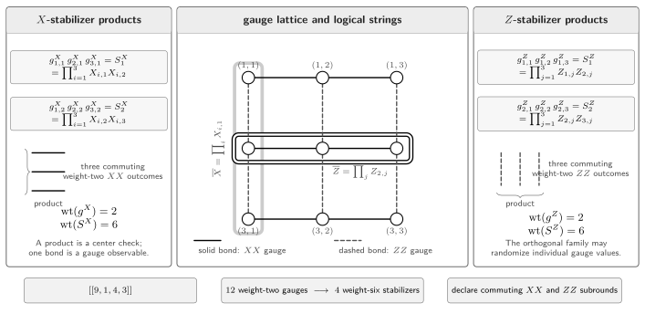
Gauge, stabilizer, and logical structure of the $[[9,1,4,3]]$ Bacon–Shor code in the convention used here. Horizontal solid bonds are weight-two $XX$ gauge generators and vertical dashed bonds are weight-two $ZZ$ gauge generators. Products of three parallel bonds across one column or row gap yield the four weight-six stabilizers. A full-column $\overline X$ and full-row $\overline Z$ intersect once and anticommute. Crossing gauge generators cannot be assigned simultaneous eigenvalues; their outcomes require declared subrounds before stabilizer parities are inferred.

Quantity	General $L\times L$ code	$3\times3$ fixture	Interpretation
physical qubits $n$	$L^2$	$9$	one at each lattice site
protected qubits $k$	$1$	$1$	one logical row-column pair
gauge qubits $r$	$(L-1)^2$	$4$	algebraic factors, not marked sites
independent stabilizers $s$	$2(L-1)$	$4$	two center-check orientations
gauge-generator count	$2L(L-1)$	$12$	weight-two bonds in this presentation
stabilizer weight	$2L$	$6$	product across a complete gap
static distance $d$	$L$	$3$	minimum dressed logical weight

Ideal decoding and circuit-level limits

At the stabilizer level, the square code reduces each Pauli sector to a repetition-code problem. A $Z$ error at column $j$ changes the adjacent $X$-stabilizer parities; an $X$ error at row $i$ changes the adjacent $Z$-stabilizer parities. With perfect syndrome extraction and an independent Pauli model, majority logic identifies a likely row or column class. The recovery need not locate the exact site, because gauge-related sites have the same protected effect.

For example, two single-qubit $X$ errors in the same row differ by a product of horizontal $XX$ gauge generators. A correction placed elsewhere in that gauge-equivalent row can restore the protected subsystem even while changing the gauge state. A correction in the wrong logical row class, by contrast, can complete a full $\overline X$ or $\overline Z$ string and fail logically.

This simple majority picture is not a circuit-level decoder. Measurement faults require repeated rounds; an ancilla fault can spread through a parity circuit; and the noncommuting gauge families impose a schedule. Aliferis and Cross (2007) constructed a fault-tolerant Bacon–Shor scheme with specific nearest-neighbor two-qubit measurements and obtained a model-specific threshold. Its numerical value is not a property of the abstract $[[9,1,4,3]]$ code. Direct stabilizer measurement, flags, subsystem-surface schedules, and hardware-native parity primitives can change the comparison.

Families and Design Tradeoffs

Generalized Bacon–Shor and compass codes

Bacon and Casaccino (2006) generalized the construction using two classical linear codes. Bravyi (2011) described a particularly transparent binary-matrix form: place a qubit at each nonzero entry of a binary matrix $A$, use $XX$ gauge generators between occupied cells in a row and $ZZ$ generators between occupied cells in a column, and obtain parameters controlled by the rank and row- and column-code distances of $A$. The full square Bacon–Shor code is one member of this larger family.

Li, Miller, Newman, Wu, and Brown (2019) organized related gauge-fixing patterns as two-dimensional compass codes. Different patterns interpolate between Bacon–Shor- and surface-code-like structures and can be tailored to asymmetric or spatially inhomogeneous noise. The chosen gauge changes which checks are measured and which equivalences the decoder uses. It does not license a performance ranking without matching circuits and noise.

Recent constructions emphasize that subsystem freedom is a general weight-and-connectivity transformation, not only a lattice curiosity. Baspin and Williamson’s 2026 wire codes map stabilizer codes to subsystem codes with weight-three, degree-three gauge interactions on a chosen graph, paying embedding-dependent qubit overhead and distance loss. The result illustrates the recurring bargain: local or sparse gauge interactions are purchased with additional gauge structure and must be assessed end to end.

Subsystem surface and color-code families

Topological subsystem codes combine geometrically local gauge measurements with nonlocal protected information. Bombín (2010) constructed two-dimensional examples with two-body gauge checks. Suchara, Bravyi, and Terhal (2011) and Bravyi, Duclos-Cianci, Poulin, and Suchara (2013) developed concrete topological subsystem and subsystem-surface constructions, including three-qubit check operators and model-specific decoding thresholds.

These families are not ordinary surface or color codes with renamed stabilizers. Their stabilizer generators can be larger than their local gauge generators, and their syndrome schedule may contain noncommuting subrounds. Surface Code owns the standard planar stabilizer architecture, while Topological Codes owns homology, local indistinguishability, active-versus-passive protection, and the common locality taxonomy.

Gauge color codes use gauge fixing to expose different transversal gates. Bombín’s 2015 gauge-color construction is the canonical research example, but Color Codes retains the 2-colex stabilizer construction, colored boundaries, decoding, and experimental record. The present page supplies the general gauge algebra; it does not reproduce a gauge-color lattice or gate protocol.

Spatial locality bounds

“Local gauge generators” and “local stabilizers” are different hypotheses. For two-dimensional subsystem codes arranged on a Euclidean lattice with bounded-range, bounded-density gauge generators, Bravyi (2011) proved

$$kd=O(n), \qquad d^2=O(n).$$

The first bound permits asymptotic behavior unavailable to the corresponding class of local commuting-projector stabilizer codes. Bravyi also established nonconstructive families with $k$ and $d$ both proportional to $\sqrt n$. If both the gauge and stabilizer groups admit spatially local generators, the stronger stabilizer-like tradeoff

$$kd^2=O(n)$$

applies under the paper’s hypotheses. None of these statements follows from bounded Pauli weight without geometry, and none applies automatically to non-Euclidean connectivity or arbitrary approximate codes.

This distinction also keeps subsystem codes separate from the stabilizer-based definition used by Quantum LDPC Codes. A Bacon–Shor presentation has weight-two gauge generators but weight-$2L$ stabilizers. Calling it qLDPC requires an explicitly broader gauge-LDPC definition; it is not qLDPC under a definition requiring bounded-weight stabilizer generators.

Evidence and implementation boundaries

Subsystem-code evidence spans theory, finite experiments, and hardware-specific comparisons. These layers should not be collapsed:

• Egan and collaborators (2021) used one finite thirteen-ion Bacon–Shor block and specific trapped-ion circuits under native device noise to demonstrate fault-tolerant preparation, measurement, a logical Clifford rotation, and a fault-tolerant stabilizer-measurement primitive. Results used offline error correction rather than intermediate measurement or a repeated-round decoder. Separate error-detection metrics postselected on $+1$ stabilizer outcomes, and some runs also discarded shots flagged by idle-qubit crosstalk detection; neither selection rule supplies scaling evidence. The record is finite logical control, not repeated stabilization or a scalable threshold.
• Sundaresan and collaborators (2023) ran up to ten syndrome rounds on one distance-three heavy-hex subsystem block using a specific flagged syndrome-extraction circuit with conditional real-time reset under native superconducting-device noise, together with matching and maximum-likelihood decoders. Some metrics used explicit leakage postselection. The finite block, round count, selection rule, and decoder remain part of the result; it is not a threshold-scaling demonstration.
• Higgott and Breuckmann (2021) simulated growing subsystem-toric instances with explicit three-qubit-check circuits under circuit-level depolarizing noise. Their schedule-aware decoder used extra gauge-fixing information and raised the reported threshold from $0.67\%$ to $0.81\%$ without an experimental selection rule. The family, circuit, noise, decoder, and asymptotic simulation are inseparable from those numbers.
• Benito and collaborators (2025) compared explicit syndrome-extraction circuits for routed surface-code, heavy-hex subsystem, and Floquet strategies on heavy-hex connectivity through finite-size Pauli-frame simulations, using minimum-weight perfect-matching decoding under documented circuit-level and IBM-calibrated noise models; no experimental selection rule was involved. Across the declared finite-size fits and qubit-footprint objective, an optimized routed surface-code strategy was most promising. This is useful negative evidence against blanket connectivity claims, not a family-independent no-go result.

Active directions should keep their dates and changed definitions visible. Alam and Rieffel (2025) use a periodic measurement schedule to obtain dynamical logical qubits in Bacon–Shor. Their schedule-dependent logical content must not be substituted for the static $[[L^2,1,(L-1)^2,L]]$ parameters derived above. Williamson and Yoder (2026) temporarily gauge a logical Pauli to implement a fault-tolerant measurement with auxiliary-qubit overhead linear in the measured operator’s weight up to a polylogarithmic factor. That is a code-deformation mechanism, not a claim that arbitrary logical measurements become free.

Gauge Fixing

Algebraic change of gauge

Gauge fixing selects a compatible commuting projective subset $\overline{\mathcal F}\subseteq\overline{\mathcal G}$ and promotes measured, signed lifts to stabilizer constraints. Algebraically,

$$\overline{\mathcal S}' = \langle\overline{\mathcal S},\overline{\mathcal F}\rangle, \qquad \overline{\mathcal G}' = \overline{\mathcal G}\cap\overline{\mathcal F}^{\perp}.$$

The second operation removes gauge directions that anticommute with the fixed operators. In a canonical gauge basis, fixing one operator such as $Z^G_a$ removes freedom in its conjugate gauge direction. If the protected logical algebra is preserved, $k$ stays fixed while $r$ decreases and the stabilizer rank increases. Releasing that constraint reintroduces the gauge degree of freedom.

Two gauge choices can therefore describe different subspace codes embedded in a common subsystem code. A logical operation transversal in one gauge may not be transversal in another. Changing gauge can expose a useful gate, convert between code descriptions, or reinterpret a deformation or joint measurement. Vuillot and collaborators (2019) formalized code deformation and lattice surgery in this language.

An arbitrary commuting subset is not automatically a valid fixing. The new constraints must be compatible with the old protected logical algebra, their signs must define a nonempty sector, and the transition must not measure a logical observable unless that measurement is the declared task. The code distance during the transition can differ from both endpoint distances.

Fault-tolerant transitions

A fault-tolerant gauge change is a spacetime protocol. It specifies which old constraints stop being enforced, which new gauge operators are measured, how many rounds are used, how faults propagate, which detector events are formed, and how the final Pauli or gauge frame is updated. If measurement errors can masquerade as a logical transition, the algebraic inclusion of groups is not enough.

Fault-Tolerant Gates is the canonical home for this operational mechanism, including gauge-color gates, code switching, deformation, and conversion faults. This page retains the algebraic reason gauge fixing can preserve the protected subsystem. Lattice Surgery owns detailed patch-parity protocols rather than the general subsystem quotient.

Single-shot correction is a still stronger property. It requires sufficient local redundancy and confinement structure to control measurement noise from one noisy round; it is not supplied by gauge qubits alone. In a separate analysis, Bombín’s 2015 single-shot study showed that three-dimensional gauge-color codes exhibit this property under specific locality and confinement hypotheses, while two-dimensional Bacon–Shor does not acquire it merely from weight-two checks.

Auditing a Subsystem-Code Claim

A claim-layer checklist

A subsystem-code claim is complete only when its conclusion matches its supporting layer. The following ledger prevents an algebraic convenience from turning into an architecture claim.

Claim layer	Minimum supporting record	Invalid shortcut
protected subsystem	explicit $\mathcal H_L\otimes\mathcal H_G$ or gauge presentation	calling unwanted behavior “gauge” after the fact
exact correctability	declared errors and $PE_a^\dagger E_bP=I_L\otimes M_{ab}$	quoting only a code distance
code parameters	independent stabilizer and gauge ranks plus logical quotients	counting listed, dependent generators
static distance	minimum dressed logical class in $\overline{\mathcal S}^{\perp}/\overline{\mathcal G}$	weight of one preferred bare logical
syndrome inference	signed gauge products and a compatible measurement schedule	multiplying arbitrary noncommuting outcomes
extraction advantage	complete circuits, locations, connectivity, ancillas, resets, and leakage	comparing check weights alone
decoder result	raw record, gauge preprocessing, prior, latency, and failure definition	using a stabilizer-only decoder unchanged
threshold	growing family, circuit/noise model, decoder, and asymptotic quantifiers	transporting a published percentage
experiment	finite sizes, rounds, selection, correction timing, and uncertainty	calling one logical operation scalable fault tolerance
resource advantage	matched task, logical target, factories, routing, timing, and total qubits	counting only data or gauge-measurement ancillas

The audit should also state whether the logical object is static or dynamical, whether distance is data-only or circuit-level, and whether gauge outcomes are retained, compressed to stabilizers, or decoded jointly. A comparison that changes two of these conventions at once cannot attribute the result to subsystem structure alone.

Canonical handoffs

Use the following ownership map when a question grows beyond this page:

• Why Quantum Error Correction Is Possible owns the general channel correctability theorem.
• Stabilizer Formalism owns Pauli symplectic algebra, projectors, normalizers, Clifford updates, and tableaus.
• Syndrome Measurement owns physical check circuits and repeated detector records.
• Decoders owns general logical-coset inference, algorithms, calibration, and latency.
• Surface Code, Color Codes, and Quantum LDPC Codes own their concrete constructions and evidence.
• Topological Codes owns topology, homology, anyon dictionaries, passive Hamiltonian protection, and conditional locality theorems outside the subsystem-specific bounds stated here.
• Fault-Tolerant Gates owns gauge-fixing gadgets, containment criteria, and universal completion; Threshold Theorem owns asymptotic simulation claims.

The subsystem page is therefore an interface: it changes the protected object and the relevant equivalence relation, then hands the resulting circuit, decoder, family, evidence, and resource questions to their canonical owners.

Exercises

1. Recover only the protected factor

Suppose $P\mathcal H\cong\mathcal H_L\otimes\mathcal H_G$ and two errors satisfy

$$PE_0^\dagger E_1P=I_L\otimes Z_G.$$

Explain why their difference is compatible with correcting $L$, and state what would change if the right-hand side were $X_L\otimes Z_G$.

Solution

In the first case the pairwise error product acts identically on the protected factor. A recovery may distinguish the errors or leave a residual $Z_G$; both outcomes preserve $\rho_L$. The operator-QEC condition is therefore satisfied for this pair. In the second case the pairwise product contains a nontrivial $X_L$. It violates the operator-QEC condition and creates an uncorrectable logical ambiguity for the declared error span.

2. Count protected and gauge qubits

A Pauli subsystem code on $n=15$ qubits has six independent stabilizers and four anticommuting gauge pairs. Find $r$, $k$, the codespace dimension, and the binary rank of the gauge group.

Solution

Four gauge pairs mean $r=4$. Since $s+k+r=n$, $k=15-6-4=5$. The common stabilizer eigenspace has dimension $2^{k+r}=2^9$. The projective gauge rank is $s+2r=6+8=14$, equivalently $n-k+r=15-5+4=14$.

3. Distinguish bare and dressed logicals

Let $\bar L\in\overline{\mathcal G}^{\perp} \setminus\overline{\mathcal S}$ be a bare logical class and $\bar g\in\overline{\mathcal G}$. Show that $\bar L\bar g$ represents the same protected logical action, and explain why $\bar L\bar g$ need not be bare.

Solution

Every gauge representative acts as the identity on $\mathcal H_L$ and possibly nontrivially on $\mathcal H_G$. Hence $\bar L$ and $\bar L\bar g$ induce the same protected operation and belong to one class in $\overline{\mathcal S}^{\perp}/\overline{\mathcal G}$. But $\bar g$ can have nonzero symplectic product with another gauge direction, so $\bar L\bar g$ need not lie in $\overline{\mathcal G}^{\perp}$. It is then a dressed logical rather than a bare one. Gauge dressing may also reduce its physical weight, which is why distance minimizes over the dressed class.

4. Derive Bacon–Shor stabilizers

For the $3\times3$ convention on this page, multiply the three horizontal gauge generators spanning the first column gap. Write the resulting stabilizer and verify that it commutes with every vertical $ZZ$ gauge bond.

Solution

The product is

$$S^X_1 = (X_{1,1}X_{1,2})(X_{2,1}X_{2,2})(X_{3,1}X_{3,2}).$$

A vertical $ZZ$ bond lies in one column. If that column is neither 1 nor 2, the overlap is zero. If it is column 1 or 2, the bond touches two qubits on which $S^X_1$ has $X$, producing two anticommutations and an overall plus sign. Thus $S^X_1$ commutes with every vertical gauge generator. It plainly commutes with all horizontal $XX$ generators, so it lies in the gauge center.

5. Decode modulo gauge

In the $3\times3$ Bacon–Shor code, compare single-qubit errors $X_{2,1}$ and $X_{2,3}$. Show that they differ by a gauge operator and explain the recovery consequence.

Solution

Their product is

$$X_{2,1}X_{2,3} = (X_{2,1}X_{2,2})(X_{2,2}X_{2,3}),$$

the product of two horizontal $XX$ gauge generators. The two errors therefore have the same protected action modulo $\mathcal G$. A recovery need not locate the column within row 2; correcting either representative leaves at most a gauge transformation. Confusing this with equivalence across different logical row classes could instead complete a logical string.

6. Audit a measurement schedule

A proposal says, “All twelve weight-two gauge checks of the $3\times3$ code are measured simultaneously, and multiplying them gives the syndrome.” Name three missing or incorrect elements and repair the statement.

Solution

Crossing horizontal $XX$ and vertical $ZZ$ checks anticommute, so they do not have simultaneous eigenvalues. The proposal also fails to specify which three like-oriented outcomes form each signed stabilizer product and gives no circuit or time ordering. A repair is: measure a declared commuting horizontal subround, infer the two $X$-stabilizer parities from products across the two column gaps, then measure a declared vertical subround and infer the two $Z$-stabilizer parities. For noisy extraction, repeat the schedule and define detector events, ancilla circuits, resets, fault propagation, and a decoder. Other valid schedules are possible, but they must supply the same information explicitly.

7. Apply a locality bound

Could a two-dimensional Euclidean subsystem family with bounded-range, bounded-density gauge generators have $k=\Theta(n^{2/3})$ and $d=\Theta(n^{1/2})$? Use the subsystem tradeoff and state why the answer does not settle an abstract nongeometric construction.

Solution

The product would scale as $kd=\Theta(n^{7/6})$, contradicting the bound $kd=O(n)$ for the declared two-dimensional local-gauge class. The proposal is therefore impossible under those geometric and density hypotheses. An abstract subsystem code with bounded-weight but long-range gauge generators is outside the theorem; so is a construction on a different geometry unless a corresponding bound is proved. The calculation cannot be exported by replacing geometric locality with sparse incidence alone.

References

• M. S. Alam and E. Rieffel, “Dynamical logical qubits in the Bacon–Shor code,” Physical Review A 112, 022436 (2025), doi:10.1103/nfxv-3dp7, arXiv:2403.03291.
• P. Aliferis and A. W. Cross, “Subsystem fault tolerance with the Bacon–Shor code,” Physical Review Letters 98, 220502 (2007), doi:10.1103/PhysRevLett.98.220502, arXiv:quant-ph/0610063.
• D. Bacon, “Operator quantum error-correcting subsystems for self-correcting quantum memories,” Physical Review A 73, 012340 (2006), doi:10.1103/PhysRevA.73.012340, arXiv:quant-ph/0506023.
• D. Bacon and A. Casaccino, “Quantum error correcting subsystem codes from two classical linear codes,” in Proceedings of the 44th Annual Allerton Conference on Communication, Control, and Computing, 520–527 (2006), arXiv:quant-ph/0610088.
• N. Baspin and D. J. Williamson, “Wire codes,” Quantum 10, 2083 (2026), doi:10.22331/q-2026-04-24-2083, arXiv:2410.10194.
• C. Benito, E. López, B. Peropadre, and A. Bermudez, “Comparative study of quantum error correction strategies for the heavy-hexagonal lattice,” Quantum 9, 1623 (2025), doi:10.22331/q-2025-02-06-1623, arXiv:2402.02185.
• H. Bombín, “Topological subsystem codes,” Physical Review A 81, 032301 (2010), doi:10.1103/PhysRevA.81.032301, arXiv:0908.4246.
• H. Bombín, “Gauge color codes: optimal transversal gates and gauge fixing in topological stabilizer codes,” New Journal of Physics 17, 083002 (2015), doi:10.1088/1367-2630/17/8/083002, arXiv:1311.0879.
• H. Bombín, “Single-shot fault-tolerant quantum error correction,” Physical Review X 5, 031043 (2015), doi:10.1103/PhysRevX.5.031043, arXiv:1404.5504.
• S. Bravyi, “Subsystem codes with spatially local generators,” Physical Review A 83, 012320 (2011), doi:10.1103/PhysRevA.83.012320, arXiv:1008.1029.
• S. Bravyi, G. Duclos-Cianci, D. Poulin, and M. Suchara, “Subsystem surface codes with three-qubit check operators,” Quantum Information and Computation 13, 963–985 (2013), doi:10.26421/QIC13.11-12-4, arXiv:1207.1443.
• L. Egan et al., “Fault-tolerant control of an error-corrected qubit,” Nature 598, 281–286 (2021), doi:10.1038/s41586-021-03928-y, arXiv:2009.11482.
• O. Higgott and N. P. Breuckmann, “Subsystem codes with high thresholds by gauge fixing and reduced qubit overhead,” Physical Review X 11, 031039 (2021), doi:10.1103/PhysRevX.11.031039, arXiv:2010.09626.
• D. W. Kribs, R. Laflamme, D. Poulin, and M. Lesosky, “Operator quantum error correction,” Quantum Information and Computation 6, 382–399 (2006), doi:10.26421/QIC6.4-5-6, arXiv:quant-ph/0504189.
• M. Li, D. Miller, and K. R. Brown, “Direct measurement of Bacon–Shor code stabilizers,” Physical Review A 98, 050301(R) (2018), doi:10.1103/PhysRevA.98.050301, arXiv:1804.01127.
• M. Li, D. Miller, M. Newman, Y. Wu, and K. R. Brown, “2D compass codes,” Physical Review X 9, 021041 (2019), doi:10.1103/PhysRevX.9.021041, arXiv:1809.01193.
• J. Napp and J. Preskill, “Optimal Bacon–Shor codes,” Quantum Information and Computation 13, 490–510 (2013), doi:10.26421/QIC13.5-6-9, arXiv:1209.0794.
• M. A. Nielsen and D. Poulin, “Algebraic and information-theoretic conditions for operator quantum error-correction,” Physical Review A 75, 064304(R) (2007), doi:10.1103/PhysRevA.75.064304, arXiv:quant-ph/0506069.
• D. Poulin, “Stabilizer formalism for operator quantum error correction,” Physical Review Letters 95, 230504 (2005), doi:10.1103/PhysRevLett.95.230504, arXiv:quant-ph/0508131.
• M. Suchara, S. Bravyi, and B. M. Terhal, “Constructions and noise threshold of topological subsystem codes,” Journal of Physics A: Mathematical and Theoretical 44, 155301 (2011), doi:10.1088/1751-8113/44/15/155301, arXiv:1012.0425.
• N. Sundaresan et al., “Demonstrating multi-round subsystem quantum error correction using matching and maximum likelihood decoders,” Nature Communications 14, 2852 (2023), doi:10.1038/s41467-023-38247-5.
• C. Vuillot, L. Lao, B. Criger, C. García Almudéver, K. Bertels, and B. M. Terhal, “Code deformation and lattice surgery are gauge fixing,” New Journal of Physics 21, 033028 (2019), doi:10.1088/1367-2630/ab0199, arXiv:1810.10037.
• D. J. Williamson and T. J. Yoder, “Low-overhead fault-tolerant quantum computation by gauging logical operators,” Nature Physics 22, 598–603 (2026), doi:10.1038/s41567-026-03220-8, arXiv:2410.02213.