Threshold Theorem

The quantum accuracy-threshold theorem says that noisy quantum hardware can simulate an arbitrarily long ideal quantum computation to arbitrarily high accuracy, provided that the noise is weaker than a positive constant and satisfies the locality assumptions of a fault-tolerant construction. The extra physical work grows only polylogarithmically with the ideal circuit size and the inverse target error in the standard concatenated-code theorem.

This is an asymptotic existence and efficiency result. It overturns the naive expectation that the error of an $L$-location circuit must grow as $Lp$, forcing the physical error strength $p$ to shrink as $1/L$. Fault-tolerant simulation instead replaces a physical location by a protected gadget whose effective failure strength decreases recursively:

$$p \longmapsto p^{(1)} \longmapsto p^{(2)} \longmapsto \cdots, \qquad p^{(j+1)} \lesssim A\bigl(p^{(j)}\bigr)^{t+1}.$$

The theorem is conditional in a precise sense. A code, gadget set, decoder or recovery rule, architecture, noise class, and error metric must be fixed before the phrase the threshold has a mathematical meaning. A measured gate fidelity below a familiar percentage is not, by itself, a theorem hypothesis.

Canonical Scope

Why Quantum Error Correction Is Possible owns the Knill–Laflamme condition and the logic by which syndromes reveal errors without revealing an unknown logical state. Fault-Tolerant Gates owns the gadget-level error-containment contract. Surface Code owns surface-code geometry, repeated syndrome extraction, and code-specific threshold scaling; Decoders owns inference algorithms and decoder benchmarks.

This page is the canonical home for the threshold theorem’s quantifiers, noise assumptions, extended-rectangle proof, recursive suppression, polylogarithmic overhead, threshold taxonomy, and limitations. Concrete algorithm-to-hardware budgets belong with Resource Estimation, while estimator software and reproducibility belong with Resource Estimation Tools. Dated device claims belong with Error-Correction Case Studies and the Fault-Tolerant Quantum Computing Frontier.

The existence of positive thresholds under stated assumptions is established mathematics. Obtaining a useful threshold and affordable overhead for a particular hardware stack remains a code-and-architecture-dependent engineering problem.

Quantum Error Correction and Fault Tolerance invokes this theorem layer only after the code, gadgets, decoder, locality, noise, and error metric are frozen; this page retains theorem quantifiers, extended-rectangle and recursive-suppression arguments, noise assumptions, threshold meanings, overhead, and limitations.

From an Ideal Circuit to a Noisy Simulation

Let $\mathcal C$ be an ideal circuit built from a fixed finite universal instruction set. Its locations include every operation at which noise may act:

• state preparations;
• one- and two-qubit gates;
• measurements and resets;
• idle or transport intervals;
• classically controlled quantum operations.

Write $L$ for the number of ideal locations, $D$ for circuit depth, and $Q$ for the maximum number of live ideal qubits. If each implementation differs from its ideal channel by worst-case error at most $\delta$, a telescoping bound gives

$$\frac12 \left\| \widetilde{\mathcal C}-\mathcal C \right\|_\diamond \leq \sum_{\ell=1}^{L} \frac12 \left\| \widetilde{\mathcal L}_{\ell} -\mathcal L_{\ell} \right\|_\diamond \leq L\delta.$$

Without active protection, keeping the total simulation error below $\varepsilon$ therefore appears to require

$$\delta \lesssim \frac{\varepsilon}{L}.$$

That requirement becomes more severe as the computation grows. The threshold theorem replaces it with a constant hardware target. The physical noise must be below a scheme-dependent threshold, but it does not need to decrease with $L$; the encoding scale is increased instead.

Operational accuracy

The output guarantee can be stated in several compatible ways. If the final answer is classical, one may require total-variation distance

$$D_{\mathrm{TV}} \bigl(P_{\mathrm{FT}},P_{\mathrm{id}}\bigr) = \frac12 \sum_x \left| P_{\mathrm{FT}}(x)-P_{\mathrm{id}}(x) \right| \leq \varepsilon.$$

For quantum output, trace distance may be used:

$$D_{\mathrm{tr}} \bigl(\rho_{\mathrm{FT}},\rho_{\mathrm{id}}\bigr) = \frac12 \left\| \rho_{\mathrm{FT}}-\rho_{\mathrm{id}} \right\|_1 \leq \varepsilon.$$

A composable circuit theorem may instead bound a channel norm such as the diamond norm. These are not interchangeable numerical conventions. The chosen theorem and its physical-noise estimate must use compatible metrics.

Schematic Theorem Statement

Fix:

1. an ideal instruction set $\mathcal G$;
2. an encoding and complete fault-tolerant simulation scheme $\mathcal S$;
3. an architecture and allowed parallel schedule;
4. a parameterized noise class $\mathcal N(p)$;
5. an operational error criterion.

Under the hypotheses of a threshold proof, there is a constant $p_{\mathrm{th}}>0$ such that, for every $p<p_{\mathrm{th}}$, every ideal circuit $\mathcal C$ of finite size $L$, and every target $\varepsilon>0$, an encoded noisy circuit $\mathcal C_{\mathrm{FT}}$ exists whose output differs from the ideal output by at most $\varepsilon$. Schematically, the order of quantifiers is

$$\underbrace{ \bigl( \mathcal G,\mathcal S,\mathcal N, \text{architecture},\text{metric} \bigr) }_{\text{fixed}} \Longrightarrow \exists\,p_{\mathrm{th}}>0\ \forall\,p<p_{\mathrm{th}}\ \forall\,(\mathcal C,\varepsilon)\ \exists\,\mathcal C_{\mathrm{FT}}.$$

For the standard concatenated-code construction, constants $c_L,c_D,c_Q,\alpha,\beta,\gamma$ exist such that one can arrange bounds of the form

$$\begin{aligned} L_{\mathrm{FT}} &\leq c_L L \left[ \log\!\left(\frac{L}{\varepsilon}\right) \right]^\alpha, \\ D_{\mathrm{FT}} &\leq c_D D \left[ \log\!\left(\frac{L}{\varepsilon}\right) \right]^\beta, \\ Q_{\mathrm{FT}} &\leq c_Q Q \left[ \log\!\left(\frac{L}{\varepsilon}\right) \right]^\gamma. \end{aligned}$$

The constants and exponents are properties of the construction, not universal numbers. Some theorem variants change the overhead statement, the allowed noise, the architecture, or the simulation metric.

The durable conclusion

Local noise below a positive, model-dependent constant is not a fundamental obstruction to arbitrarily reliable quantum computation. The theorem does not say that every noise process with a small reported average error is local, nor that the resulting overhead is practical.

Why Error Correction Alone Is Insufficient

An ideal code of distance

$$d=2t+1$$

corrects every error on at most $t$ physical qubits in a block. But an actual recovery circuit contains faulty gates, measurements, ancillas, idles, and feedforward. A single fault can spread through a poorly designed circuit and create more than $t$ data errors. Repeating ideal correction more often does not solve that problem.

A fault-tolerant gadget is designed so that a small number of internal faults cannot produce an uncorrectable output. In schematic form, the gadget properties ensure that whenever the total number of incoming errors and new faults is at most $t$:

• error correction returns the block to the correct logical state, possibly with a bounded number of residual physical errors;
• an encoded gate maps correctable input errors and gadget faults to correctable output errors;
• preparation and measurement have corresponding encoded correctness properties;
• error propagation between code blocks remains bounded.

These properties convert code distance into a statement about faulty circuits. They are the local lemmas from which a global threshold proof is built.

Rectangles and Extended Rectangles

Protected replacements

At level 1 of a concatenated simulation, each ideal location is replaced by an encoded gadget. A rectangle consists of the logical operation followed by error correction on its output blocks. An extended rectangle, abbreviated exRec, also includes the leading error correction on its input blocks.

The leading correction handles errors inherited from the previous gadget. The trailing correction becomes the leading correction of the next exRec, so adjacent exRecs overlap. Preparations and measurements use modified endpoint definitions, but the same inductive purpose.

Introduce an ideal decoder only as a mathematical comparison map. A correct exRec obeys a relation of the form

$$\mathsf{Dec} \circ \mathrm{exRec}_{U} \simeq U \circ \mathsf{Dec},$$

where $\simeq$ means equality of the decoded logical action under the proof’s declared fault conditions. The physical implementation need not run this ideal decoder.

Good and bad exRecs

For a distance-$2t+1$ construction satisfying the gadget properties:

• an exRec containing at most $t$ suitably located faults is good;
• a good exRec is correct;
• therefore an incorrect, or bad, exRec requires at least $t+1$ faults.

The phrase suitably located matters. Not every set of $t+1$ faults causes a logical failure, and some proof variants classify faults by type. A set of locations is malignant if adversarial faults at those locations can make the exRec incorrect after decoding.

If an exRec contains $M$ elementary locations and $A_r$ of its $r$-location subsets are malignant, then independent stochastic noise gives the union bound

$$p^{(1)} \leq \sum_{r=t+1}^{M} A_r p^r.$$

Counting every subset would replace $A_r$ by $\binom Mr$ and usually produce a much weaker bound. Malignant-set counting improves a rigorous sufficient threshold without changing the proof’s logic.

Overlap and truncation

Because neighboring exRecs share an error-correction gadget, their badness events are not automatically disjoint. A proof cannot simply multiply independent failure probabilities. The extended-rectangle method resolves this by processing exRecs in circuit order and truncating a shared correction when required. Correctness lemmas are formulated so that each retained bad exRec can be associated with enough underlying faults.

This bookkeeping is not cosmetic. It is what makes recursive level reduction valid: contract every level-1 exRec to one effective location and obtain a circuit with the same ideal structure but a smaller effective noise strength.

Recursive Suppression

Let

$$s=t+1.$$

Suppose a simplified malignant-set estimate gives

$$p^{(j+1)} \leq A\bigl(p^{(j)}\bigr)^s, \qquad p^{(0)}=p.$$

The nonzero fixed point of the equality is

$$p_{\mathrm{th}} = A^{-1/(s-1)} = A^{-1/t}.$$

Since

$$A p_{\mathrm{th}}^{\,s-1}=1,$$

the normalized recurrence satisfies

$$\frac{p^{(j+1)}}{p_{\mathrm{th}}} \leq \left( \frac{p^{(j)}}{p_{\mathrm{th}}} \right)^s.$$

Iteration yields the characteristic doubly exponential suppression in concatenation level:

$$p^{(k)} \leq p_{\mathrm{th}} \left( \frac{p}{p_{\mathrm{th}}} \right)^{s^k}.$$

For a distance-three code, $t=1$ and $s=2$, so

$$p^{(k)} \leq p_{\mathrm{th}} \left( \frac{p}{p_{\mathrm{th}}} \right)^{2^k}.$$

The realistic recurrence is a polynomial

$$F(x) = \sum_{r=t+1}^{M} A_r x^r, \qquad p^{(j+1)} \leq F\!\left(p^{(j)}\right).$$

A rigorous sufficient threshold is any interval on which

$$F(x)<x.$$

The actual critical value of a complete scheme can be higher than a conservative proof bound.

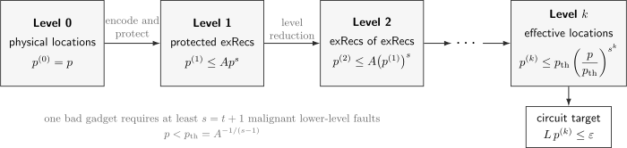
At each concatenation level, a protected gadget is contracted to one effective location. If an incorrect distance-$2t+1$ gadget requires at least $t+1$ malignant lower-level faults, then $p^{(j+1)}\lesssim A(p^{(j)})^{t+1}$. Below $p_{\mathrm{th}}$, enough levels make the circuit contribution $L p^{(k)}$ smaller than the target $\varepsilon$.

Choosing the number of levels

A union bound over $L$ effective ideal locations gives

$$p_{\mathrm{fail}} \leq L p^{(k)}.$$

It is enough to choose $k$ so that

$$L p_{\mathrm{th}} \left( \frac{p}{p_{\mathrm{th}}} \right)^{s^k} \leq \varepsilon.$$

For $p<p_{\mathrm{th}}$, this is achieved by

$$k \geq \log_s \left[ \frac{ \log\!\left(Lp_{\mathrm{th}}/\varepsilon\right) }{ \log\!\left(p_{\mathrm{th}}/p\right) } \right],$$

with a ceiling and $k\geq0$ understood. Thus

$$k = O\!\left( \log\log\frac{L}{\varepsilon} \right)$$

at fixed subthreshold $p$. A logarithmically small number of concatenation levels is enough because the effective fault strength falls doubly exponentially in $k$.

Noise Assumptions

The phrase error rate $p$ is incomplete until it is attached to a noise model. Threshold theorems are robust to more than independent Pauli flips, but they do not cover arbitrary correlations merely because each individual location looks accurate.

Independent stochastic faults

In the simplest circuit-level model, each location is faulty independently with probability at most $p$. Conditioned on the faulty locations, the faulty operations may be stochastic Pauli channels or arbitrary adversarial channels, depending on the theorem.

Independence makes the probability that a specified set $S$ of locations is faulty no larger than

$$\Pr(S\subseteq E) \leq p^{|S|},$$

where $E$ is the random fault set.

Local stochastic faults

The same inequality can be adopted as the definition of local stochastic noise:

$$\Pr(S\subseteq E) \leq p^{|S|} \qquad \text{for every finite set }S.$$

This model permits correlations. It constrains their tails: forcing faults at $r$ specified locations must cost at least a factor comparable to $p^r$. The faults need not have identical marginals, and the conditional operation at a faulty set can be adversarial.

Local stochasticity is stronger than saying that every single location has error probability at most $p$. Consider a common-mode event that, with probability $q$, faults all $N$ active qubits. Every location has marginal error $q$, but for any $r$-location set

$$\Pr(S\subseteq E)=q,$$

not $q^r$. For fixed $q>0$, no size-independent local-stochastic parameter $p<1$ can satisfy the required bound for arbitrarily large $r$.

Coherent and non-Markovian noise

A stochastic fault set is not the only route to a theorem. In a coherent fault-path expansion, write the joint system–environment evolution as

$$U_{\mathrm{noisy}} = E_{\varnothing} + \sum_{\varnothing\neq R} E_R,$$

where $E_{\varnothing}$ is the no-fault history, with the intended system action and any allowed bath evolution, and $E_R$ collects histories with faults at the locations in $R$. A local noise condition can bound the norm of all histories faulty on at least a specified set $S$:

$$\left\| \sum_{R\supseteq S} E_R \right\| \leq \eta^{|S|}.$$

Here $\eta$ is an error amplitude, not necessarily a failure probability or average infidelity. The level-reduction argument then bounds sums of bad fault paths in norm. Interference between paths changes the constants and requires amplitude bookkeeping rather than an ordinary probability union bound.

Microscopic variants start from a Hamiltonian such as

$$H(t) = H_{\mathrm S}(t) + H_{\mathrm B} + \sum_a H_{\mathrm{SB},a}(t),$$

where each $H_{\mathrm{SB},a}$ couples the bath only to qubits participating in one elementary location. A dimensionless strength can scale like

$$\eta \sim t_0 \max_a \left\| H_{\mathrm{SB},a} \right\|,$$

with $t_0$ an elementary gate time. Specific theorems also allow selected spatial correlations, including pair couplings that decay sufficiently fast with separation. Such results are not licenses for arbitrary collective noise; their norm and decay hypotheses are part of the theorem.

Leakage and loss

Ordinary qubit proofs assume faults remain in the computational space. Leakage instead uses

$$\mathcal H_{\mathrm{phys}} = \mathcal H_{\mathrm{comp}} \oplus \mathcal H_{\mathrm{leak}}.$$

A leaked control can corrupt several later targets unless the gadget limits its lifetime. Leakage threshold theorems insert or absorb leakage-reduction units, such as teleportation or reset-and-replace operations, so a local leakage fault is converted into a bounded ordinary fault with modified constants.

Loss can be easier when its location is reliably heralded, because a known erasure is less ambiguous than an unknown Pauli fault. But loss detection, replacement, delayed flags, false flags, and transport errors must be part of the location model. Calling loss an erasure does not make its handling free.

Geometry, timing, and classical control

A theorem must also declare whether:

• any pair of qubits may interact or only geometric neighbors;
• gates and checks may run in parallel;
• measurement and reset have bounded latency;
• fresh ancillas are available;
• classical decoding and feedforward are perfect, noisy, instantaneous, or explicitly scheduled;
• qubits can wait without an error cost that grows with system size;
• crosstalk remains local as more operations run simultaneously.

Thresholds survive several locality restrictions, but the gadgets and overhead change. A proof for nonlocal transversal interactions cannot simply be assigned to a two-dimensional nearest-neighbor layout without routing faults and idle time.

What Locality Really Excludes

The required locality is about fault strength, not merely geometric distance. Short-range hardware can still generate strongly correlated faults through shared control lines, resonators, laser beams, calibration parameters, cosmic-ray events, or decoder feedback. Conversely, a model with spatially long-range interactions can satisfy a threshold theorem when joint fault-path amplitudes decay sufficiently rapidly.

Three questions should be kept separate:

1. Does the microscopic noise obey a proved locality bound?
2. Does a fitted effective circuit model approximate the relevant experiment?
3. Does the implemented decoder exploit or ignore the correlations that remain?

A convincing threshold claim answers all three. Agreement of a few marginal error rates does not determine the high-weight tail that controls logical failure.

Threshold Concept Versus Threshold Value

The threshold concept is the existence of a nonzero subthreshold region in which increasing the encoding scale suppresses logical error with efficient overhead. A threshold value is a boundary in one specified model and parameterization.

Real circuit noise is a vector,

$$\boldsymbol p = \bigl( p_{\mathrm{1q}}, p_{\mathrm{2q}}, p_{\mathrm{prep}}, p_{\mathrm{meas}}, p_{\mathrm{idle}}, p_{\mathrm{loss}}, \ldots \bigr),$$

possibly augmented by bias, correlation, leakage, and timing parameters. The subthreshold object is therefore a region

$$\Omega_{\mathrm{FT}} = \left\{ \boldsymbol p: p_{\mathrm L} \longrightarrow 0 \text{ as the code scale increases} \right\}.$$

A single quoted number usually comes from restricting to a ray

$$\boldsymbol p(\lambda) = \lambda\boldsymbol r$$

with fixed relative rates $\boldsymbol r$, then finding the largest $\lambda$ for which suppression persists. Change $\boldsymbol r$, the decoder, the circuit schedule, or the logical metric, and the quoted number changes.

Term	What it means	What it does not automatically mean
rigorous lower bound	a proof-certified sufficient noise strength	the actual critical value
asymptotic threshold	a critical boundary for a fixed scaling family and model	a finite-device break-even point
simulated threshold	a numerical estimate under a specified sampler, decoder, and fit	a theorem for unmodeled hardware noise
finite-size crossing	an intersection of logical-error curves at tested sizes	the infinite-size critical point
pseudothreshold	where one encoded construction matches a chosen lower-level or physical reference	the recursive or asymptotic threshold
experimental below-threshold evidence	logical error decreases across matched implemented code scales	a complete universal fault-tolerant computer

A proved lower bound is one-sided

If a theorem establishes

$$p_{\mathrm{th}} \geq p_{\mathrm{LB}},$$

then $p<p_{\mathrm{LB}}$ is sufficient under its hypotheses. The case $p>p_{\mathrm{LB}}$ is undecided by that proof. It does not imply failure. Conversely, a high numerical threshold under an idealized Pauli model does not prove that hardware with the same average infidelity lies in the modeled subthreshold region.

Pseudothresholds depend on the operation

For one level of encoding, a pseudothreshold may solve

$$p_{\mathrm L}^{(1)}(p_\star)=p_\star.$$

But state preparation, memory, CNOT, logical parity measurement, and magic state injection can have different curves and different pseudothresholds. Level-1 crossings may move under further concatenation. An exRec pseudothreshold can be a useful diagnostic while still differing from the asymptotic accuracy threshold.

Matching Experimental Metrics to Theorem Parameters

Average gate infidelity, randomized-benchmarking error per Clifford, cycle error, Pauli error probability, diamond distance, leakage probability, and fault-path amplitude are different quantities. A threshold parameter cannot be replaced by whichever measured scalar is smallest.

For a coherent qubit overrotation

$$U_\theta = \exp\!\left( -\frac{i\theta Z}{2} \right),$$

the average gate infidelity relative to the identity is

$$r_{\mathrm{avg}} = \frac{2}{3} \sin^2\!\left(\frac{\theta}{2}\right) \approx \frac{\theta^2}{6},$$

whereas the half diamond distance is

$$\delta_\diamond = \frac12 \left\| \mathcal U_\theta-\mathcal I \right\|_\diamond = \left| \sin\!\left(\frac{\theta}{2}\right) \right| \approx \frac{|\theta|}{2}.$$

The worst-case error is first order in $|\theta|$ while average infidelity is second order. Stochastic Pauli noise has a more favorable relation between these metrics. Randomized compiling or tailored decoding may reduce coherent accumulation, but that transformed process and its residual correlations must be justified rather than assumed.

Overhead Scaling

Concatenated-code overhead

Suppose each level replaces one lower-level location by at most $G$ locations, has gadget depth at most $H$, and replaces each lower-level data qubit by at most $n$ qubits including its allocated ancillas. Then

$$\begin{aligned} L_k &\leq L G^k,\\ D_k &\leq D H^k,\\ Q_k &\leq Q n^k. \end{aligned}$$

Using

$$k = O\!\left( \log\log\frac{L}{\varepsilon} \right)$$

gives

$$\begin{aligned} L_k &= O\!\left[ L \left( \log\frac{L}{\varepsilon} \right)^{\log_s G} \right], \\ D_k &= O\!\left[ D \left( \log\frac{L}{\varepsilon} \right)^{\log_s H} \right], \\ Q_k &= O\!\left[ Q \left( \log\frac{L}{\varepsilon} \right)^{\log_s n} \right]. \end{aligned}$$

This is the origin of polylogarithmic overhead in the standard theorem. It is an asymptotic scaling statement. The constants hidden in the notation can include verified ancilla preparation, rejected attempts, routing, idles, decoder work, and non-Clifford resources.

Near-threshold overhead

The level requirement contains

$$\log\!\left( \frac{p_{\mathrm{th}}}{p} \right)$$

in the denominator. As $p$ approaches $p_{\mathrm{th}}$ from below, this quantity tends to zero and the required encoding scale can become very large. The theorem promises efficient asymptotic scaling at fixed $p<p_{\mathrm{th}}$; it does not promise a gentle engineering cost arbitrarily close to threshold.

Topological-code scaling

Topological-code proofs organize suppression by spacetime distance rather than concatenation level. Below a model-specific critical point, one often obtains a bound of the schematic form

$$p_{\mathrm L}(d) \leq \operatorname{poly}(d) \exp(-\alpha d), \qquad \alpha>0.$$

Making $L p_{\mathrm L}(d)\leq\varepsilon$ then requires

$$d = O\!\left( \log\frac{L}{\varepsilon} \right).$$

For a two-dimensional patch with $O(d^2)$ qubits and protected operations lasting $O(d)$ rounds, this again produces polylogarithmic spacetime overhead. The precise powers and constants depend on layout and operation. Surface Code and Lattice Surgery own those architectural details.

Constant overhead is a stronger result

The standard threshold theorem does not claim constant qubit overhead. Separate constructions using constant-rate quantum LDPC families can achieve asymptotically constant space overhead under additional code, decoder, connectivity, and circuit assumptions. That is a stronger theorem with a different systems contract, not a reinterpretation of the ordinary polylogarithmic result. Quantum LDPC Codes develops the code families and implementation tradeoffs.

A Worked Recursive Estimate

Consider the illustrative distance-three recurrence

$$p^{(j+1)} \leq 10^3 \bigl(p^{(j)}\bigr)^2.$$

The simplified fixed point is

$$p_{\mathrm{th}}=10^{-3}.$$

At physical strength $p=10^{-4}$,

$$\begin{aligned} p^{(1)} &\leq 10^{-5}, \\ p^{(2)} &\leq 10^{-7}, \\ p^{(3)} &\leq 10^{-11}. \end{aligned}$$

For $L=10^8$ ideal locations, the union bound at level 3 is

$$L p^{(3)} \leq 10^{-3}.$$

This example displays the mechanism, not an architecture forecast. If a level replacement uses $G=100$ lower-level locations, then three levels cost up to

$$G^3=10^6$$

physical locations per ideal location before accounting for rejected ancillas or routing. A scheme can be comfortably below threshold and still be impractical at the target problem size.

The Theorem Landscape

There is not one threshold theorem with one hypothesis list. Major proof families establish related conclusions under different contracts.

Proof family	Organizing mechanism	Representative qualification
early encoded computation	fault-tolerant recovery and recursive encoding	foundational constructions had conservative constants
concatenated codes	exRecs, malignant sets, and level reduction	polylogarithmic overhead under local stochastic or norm-bounded noise
topological codes	suppression of nontrivial spacetime fault chains	threshold depends on lattice, extraction circuit, decoder, and noise
non-Markovian models	norm bounds on coherent fault-path sums	local coupling strength replaces a simple probability
decaying long-range noise	bounds on spatially correlated interactions	decay and dimension hypotheses are essential
leakage models	leakage-reduction units convert leakage into bounded faults	reset or teleportation overhead changes constants
postselected schemes	error detection and verified ancilla acceptance	acceptance probability and correlation assumptions matter
continuous-variable schemes	finite-energy bosonic gadgets plus an outer code	energy and channel constraints replace idealized infinite squeezing
constant-overhead schemes	constant-rate codes and robust noisy-syndrome decoding	stronger code and connectivity assumptions

The historical progression matters. Shor first showed how encoded fault-tolerant circuits weakened the required decrease of component error with circuit size. Aharonov and Ben-Or, Knill, Laflamme, and Zurek, and related work established constant positive thresholds. The extended-rectangle and level-reduction framework later made recursive correctness and threshold lower bounds especially explicit for distance-three and higher-distance concatenated codes.

What the Theorem Does Not Guarantee

The theorem does not establish any of the following without additional work:

• A universal threshold number. Thresholds belong to complete models and constructions.
• That a device is below threshold. Hardware noise must be connected to the theorem’s parameter, including correlations, leakage, idles, and simultaneous operation.
• That one encoded qubit beats one physical qubit. Break-even is a finite-size comparison; a threshold is an asymptotic scaling property.
• That a memory threshold is a computation threshold. Logical gates, preparation, measurement, routing, injection, and feedforward can be the limiting operations.
• That the decoder is free. Throughput, latency, memory, calibration, and handoff across changing circuits belong inside an operational architecture.
• That a high average gate fidelity controls worst-case error. Coherent and correlated tails can dominate logical failure.
• That subthreshold error means zero error. A finite code has a nonzero logical failure probability; scale is chosen to meet an error budget.
• That operation above a proved lower bound is impossible. A lower bound is sufficient, not necessary.
• That overhead is affordable. Polylogarithmic asymptotics can hide large constants and poor near-threshold behavior.
• That universal computation is already supplied. A protected Clifford memory still needs non-Clifford resources and a complete instruction set.
• That active correction is passive self-correction. Continuous extraction, entropy removal, and control remain physical processes.
• That useful quantum advantage follows. Algorithm choice, input/output costs, runtime, and classical alternatives are separate questions.

Interpreting Below-Threshold Evidence

In experimental work, below threshold most often means that a matched logical metric improves as code scale increases under one declared circuit, decoder, and noise environment. For example, a family may show

$$p_{\mathrm L}(d+2) < p_{\mathrm L}(d)$$

with statistical confidence over the tested distances. This is meaningful evidence for scalable suppression in that operating regime.

It is not a direct laboratory proof of every microscopic assumption in a mathematical threshold theorem. A careful claim records:

• the code family and realized distances;
• the complete extraction or logical-operation circuit;
• the logical observable and denominator, such as per round or per operation;
• the decoder and whether it is online, offline, calibrated, or noise-informed;
• leakage, loss, reset, postselection, and discarded-shot treatment;
• confidence intervals and stability over acquisition time;
• whether preparations, measurements, gates, and feedforward are all inside the tested boundary.

One improved distance is evidence, not an infinite-size limit. Memory scaling does not automatically transfer to logical CNOTs or magic-state factories. Reporting Standards and Error-Correction Case Studies develop the experimental evidence ladder without changing the theorem’s canonical statement.

Common Mistakes

• Saying “the threshold is one percent” without a code, circuit, decoder, noise model, and metric.
• Substituting average gate infidelity for a stochastic or diamond-norm threshold parameter without a justified conversion.
• Counting data-gate errors while omitting preparation, measurement, reset, idle, transport, and classical-control timing.
• Assuming low one-location marginals rule out dangerous many-location bursts.
• Calling a level-1 pseudothreshold or two-distance crossing the asymptotic threshold.
• Treating a theorem lower bound as the exact critical point.
• Applying a memory threshold to a universal gate set without analyzing its logical operations.
• Using an ideal decoder in a threshold simulation and omitting its latency and mismatch from the architecture claim.
• Inferring practical resources from big-$O$ notation alone.
• Saying the theorem “corrects arbitrary errors” while dropping the locality restriction on multi-location fault strength.
• Assuming $p>p_{\mathrm{th}}$ proves that error correction can never help at finite size.
• Assuming $p<p_{\mathrm{th}}$ makes every additional encoding level helpful before constants and operation-specific pseudothresholds are checked.

A Threshold Audit Workflow

1. Define the ideal computation. Record its instruction set, size, depth, live qubits, output, and target simulation error.
2. Enumerate physical locations. Include gates, preparations, measurements, resets, waits, movement, and parallel scheduling.
3. State the noise class. Give the probability, norm, correlation, leakage, loss, and nonstationarity assumptions.
4. Match the metric. Explain how measured quantities bound the theorem’s physical-noise parameter.
5. Specify the code and gadgets. State distance, propagation rules, correction schedule, and universal logical operations.
6. Prove local correctness. Show that good exRecs or protected spacetime regions implement the intended decoded operation.
7. Bound bad structures. Count malignant fault sets or nontrivial fault chains without assuming unjustified independence.
8. Establish suppression. Derive a recursion or scale-dependent logical bound with a positive subthreshold region.
9. Allocate total failure. Choose concatenation level or distance so all logical locations fit within $\varepsilon$.
10. Account for resources. Include factories, routing, decoder latency, rejected preparations, and classical reaction time.
11. Separate proof from evidence. Label rigorous bounds, simulations, finite-size crossings, and device measurements accurately.

Further Connections

• Why Quantum Error Correction Is Possible provides the ideal recovery condition that fault-tolerant gadgets must preserve in the presence of circuit faults.
• Fault-Tolerant Gates develops transversal, deformation, gauge-fixing, pieceable, and teleportation-based mechanisms that instantiate the gadget assumptions.
• Decoders explains how model mismatch, latency, and finite-window processing affect delivered logical performance.
• GKP Codes discusses finite-energy continuous-variable threshold results and the need to state energy and channel hypotheses.
• Metrics for Quantum Hardware distinguishes average fidelity, worst-case distance, leakage, crosstalk, cycle metrics, and logical metrics.
• Logical Benchmarking designs finite-size suppression, break-even, and protected-operation tests without conflating them with an asymptotic theorem threshold.
• Resource Estimation turns an asymptotic suppression law into code distances, physical-qubit inventories, factory capacity, runtime, and failure budgets.
• Resource Estimation Tools makes that model versioned, testable, and reproducible in software.

Exercises

1. Solve the recursive threshold model

Let

$$p^{(j+1)} \leq A\bigl(p^{(j)}\bigr)^{t+1}.$$

Derive the simplified threshold $p_{\mathrm{th}}$ and prove by induction that

$$p^{(k)} \leq p_{\mathrm{th}} \left( \frac{p}{p_{\mathrm{th}}} \right)^{(t+1)^k}.$$

Solution

Set $s=t+1$. The nonzero fixed point of $x=Ax^s$ is

$$p_{\mathrm{th}} = A^{-1/(s-1)} = A^{-1/t}.$$

Therefore $A p_{\mathrm{th}}^{s-1}=1$. Defining $x_j=p^{(j)}/p_{\mathrm{th}}$ gives

$$x_{j+1} \leq x_j^s.$$

For $k=0$, $x_0=p/p_{\mathrm{th}}$. If $x_k\leq x_0^{s^k}$, then

$$x_{k+1} \leq x_k^s \leq x_0^{s^{k+1}}.$$

Induction yields the requested result. If $p<p_{\mathrm{th}}$, the base $p/p_{\mathrm{th}}$ is smaller than one, so suppression is doubly exponential in $k$.

2. Choose a concatenation level

For a distance-three scheme, take $p/p_{\mathrm{th}}=0.1$, $p_{\mathrm{th}}=10^{-3}$, $L=10^{12}$, and target total failure $\varepsilon=10^{-6}$. Find the smallest $k$ certified by

$$L p_{\mathrm{th}} \left( \frac{p}{p_{\mathrm{th}}} \right)^{2^k} \leq \varepsilon.$$

Solution

The condition is

$$10^{12} 10^{-3} \left(10^{-1}\right)^{2^k} \leq 10^{-6},$$

or

$$10^{9-2^k} \leq 10^{-6}.$$

Thus $2^k\geq15$. Since $2^3=8$ and $2^4=16$, the smallest certified level is

$$k=4.$$

This is only the level implied by the simplified bound. A complete resource estimate must use operation-specific gadgets and failure allocations.

3. Derive the polylogarithmic size exponent

Suppose one concatenation level replaces every location by at most $G$ locations and the effective fault exponent is $s=t+1$. Show that the physical location overhead is polylogarithmic in $L/\varepsilon$ and identify its exponent.

Solution

Threshold suppression requires

$$k = O\!\left( \log_s\log\frac{L}{\varepsilon} \right).$$

The replacement cost is $G^k$. Therefore

$$\begin{aligned} G^k &= \exp(k\log G) \\ &= O\!\left[ \left( \log\frac{L}{\varepsilon} \right)^{\log_s G} \right]. \end{aligned}$$

Multiplying by the ideal size gives

$$L_{\mathrm{FT}} = O\!\left[ L \left( \log\frac{L}{\varepsilon} \right)^{\log_s G} \right].$$

The exponent $\log_s G$ depends on the gadget and code.

4. Test a correlated burst

For each circuit cycle, suppose a controller fault occurs with probability $q=10^{-6}$ and applies a $Z$ error to every active qubit. All other operations are perfect. Each qubit’s marginal error probability is $10^{-6}$. Does this family satisfy local stochastic noise with parameter $p=10^{-6}$ as the processor grows?

Solution

No. For any specified set $S$ of $r$ active qubits, the common event faults all of them, so

$$\Pr(S\subseteq E)=q=10^{-6}.$$

Local stochastic noise with $p=10^{-6}$ would require

$$\Pr(S\subseteq E) \leq p^r = 10^{-6r}.$$

The inequality already fails for $r=2$. Small one-qubit marginals do not control the high-weight tail. A theorem could still apply under another model, but this noise does not satisfy the stated local-stochastic hypothesis.

5. Distinguish three thresholds

A simulation finds that distance-3 and distance-5 memory curves cross at $0.9\%$. A level-1 encoded CNOT matches its unencoded CNOT at $0.4\%$. A rigorous malignant-set proof guarantees a threshold above $0.02\%$. What can be concluded from each number?

Solution

The $0.9\%$ value is a finite-size crossing for one memory circuit, noise model, and decoder. It may estimate an asymptotic memory threshold but is not itself a proof.

The $0.4\%$ value is an operation-specific level-1 pseudothreshold. It need not equal either the memory crossing or the recursive threshold.

The $0.02\%$ value is a rigorous sufficient lower bound under the proof’s assumptions. Noise below it is certified by that theorem. Noise above it is not certified, but the proof does not establish failure there. The three numbers answer different questions and need not agree.

6. Compare coherent-error metrics

For a small $Z$ overrotation with $\theta=10^{-3}$, estimate the average gate infidelity and half diamond distance. Why is quoting only the former potentially misleading in a threshold comparison?

Solution

Using the small-angle formulas,

$$r_{\mathrm{avg}} \approx \frac{\theta^2}{6} \approx 1.67\times10^{-7},$$

while

$$\delta_\diamond \approx \frac{|\theta|}{2} = 5.0\times10^{-4}.$$

The two metrics differ parametrically because coherent amplitude can accumulate before being randomized or detected. A theorem stated in a worst-case norm cannot use the average infidelity as its parameter without a valid conversion or a more detailed noise model.

7. Choose a topological-code distance

Assume the bound

$$p_{\mathrm L}(d) \leq 0.1e^{-0.5d}$$

per logical location. For $L=10^9$ logical locations and target $\varepsilon=10^{-3}$, find a sufficient real-valued $d$, then round up to the next odd distance.

Solution

Require

$$10^9 \left( 0.1e^{-0.5d} \right) \leq 10^{-3}.$$

Thus

$$e^{-0.5d} \leq 10^{-11},$$

and

$$d \geq 2\log(10^{11}) = 22\log 10 \approx 50.66.$$

The next odd integer is

$$d=51.$$

This answer is conditional on the bound applying to the relevant logical operation and noise model. It does not include routing, factory, or decoder costs.

8. Audit a below-threshold claim

A processor reports $99.95\%$ average two-qubit gate fidelity and cites a $1\%$ surface-code threshold. No repeated syndrome data, leakage rate, simultaneous-gate benchmark, or decoder is reported. Is “the processor is below threshold” justified?

Solution

No. The two percentages refer to unspecified or incompatible objects. A surface-code threshold belongs to a complete circuit-level noise model, schedule, decoder, and logical metric. Average isolated-gate infidelity does not determine worst-case coherent error, crosstalk, leakage, measurement, reset, idle, or correlated-fault tails.

The reported gate fidelity may be encouraging component evidence. A below-threshold system claim requires a justified map into the threshold model or matched logical suppression across increasing code scale, with the rest of the error-correction cycle inside the boundary.

References

1. P. W. Shor, “Fault-tolerant quantum computation,” in Proceedings of the 37th Annual Symposium on Foundations of Computer Science, 56–65 (1996), doi:10.1109/SFCS.1996.548464.
2. D. Aharonov and M. Ben-Or, “Fault-tolerant quantum computation with constant error rate,” SIAM Journal on Computing 38, 1207–1282 (2008), doi:10.1137/S0097539799359385.
3. E. Knill, R. Laflamme, and W. H. Zurek, “Resilient quantum computation,” Science 279, 342–345 (1998), doi:10.1126/science.279.5349.342.
4. J. Preskill, “Reliable quantum computers,” Proceedings of the Royal Society A 454, 385–410 (1998), doi:10.1098/rspa.1998.0167.
5. D. Gottesman, “Theory of fault-tolerant quantum computation,” Physical Review A 57, 127–137 (1998), doi:10.1103/PhysRevA.57.127.
6. P. Aliferis, D. Gottesman, and J. Preskill, “Quantum accuracy threshold for concatenated distance-3 codes,” Quantum Information and Computation 6, 97–165 (2006), arXiv:quant-ph/0504218.
7. B. M. Terhal and G. Burkard, “Fault-tolerant quantum computation for local non-Markovian noise,” Physical Review A 71, 012336 (2005), doi:10.1103/PhysRevA.71.012336.
8. D. Aharonov, A. Kitaev, and J. Preskill, “Fault-tolerant quantum computation with long-range correlated noise,” Physical Review Letters 96, 050504 (2006), doi:10.1103/PhysRevLett.96.050504.
9. P. Aliferis and B. M. Terhal, “Fault-tolerant quantum computation for local leakage faults,” Quantum Information and Computation 7, 139–156 (2007), arXiv:quant-ph/0511065.
10. E. Dennis, A. Kitaev, A. Landahl, and J. Preskill, “Topological quantum memory,” Journal of Mathematical Physics 43, 4452–4505 (2002), doi:10.1063/1.1499754.
11. R. Raussendorf and J. Harrington, “Fault-tolerant quantum computation with high threshold in two dimensions,” Physical Review Letters 98, 190504 (2007), doi:10.1103/PhysRevLett.98.190504.
12. R. Raussendorf, J. Harrington, and K. Goyal, “Topological fault-tolerance in cluster state quantum computation,” New Journal of Physics 9, 199 (2007), doi:10.1088/1367-2630/9/6/199.
13. P. Aliferis, D. Gottesman, and J. Preskill, “Accuracy threshold for postselected quantum computation,” Quantum Information and Computation 8, 181–244 (2008), arXiv:quant-ph/0703264.
14. J. J. Wallman, C. Granade, R. Harper, and S. T. Flammia, “Estimating the coherence of noise,” New Journal of Physics 17, 113020 (2015), doi:10.1088/1367-2630/17/11/113020.
15. D. Gottesman, “Fault-tolerant quantum computation with constant overhead,” Quantum Information and Computation 14, 1338–1372 (2014), doi:10.26421/QIC14.15-16.
16. O. Fawzi, A. Grospellier, and A. Leverrier, “Constant overhead quantum fault-tolerance with quantum expander codes,” in 2018 IEEE 59th Annual Symposium on Foundations of Computer Science, 743–754 (2018), doi:10.1109/FOCS.2018.00076.
17. A. G. Fowler, M. Mariantoni, J. M. Martinis, and A. N. Cleland, “Surface codes: Towards practical large-scale quantum computation,” Physical Review A 86, 032324 (2012), doi:10.1103/PhysRevA.86.032324.
18. R. Harper and S. T. Flammia, “Fault-tolerant logical gates in the IBM Quantum Experience,” Physical Review Letters 122, 080504 (2019), doi:10.1103/PhysRevLett.122.080504.