Error-Correction Case Studies

Short Definition

An error-correction case study follows quantum information through an implemented code, noisy syndrome circuit, classical decoder, recovery or Pauli-frame update, and final logical measurement. Its central question is not whether errors were detected. It is whether the complete procedure produced a better logical channel than a declared reference under a fair accounting of time, hardware, discarded runs, and uncertainty.

This page compares four kinds of evidence:

• repeated syndrome extraction in a one-error-type repetition code;
• finite-distance surface-code memory experiments;
• logical-lifetime comparisons against physical and uncorrected references;
• bosonic-code demonstrations in oscillator modules.

Why Quantum Error Correction Is Possible owns the Knill–Laflamme criterion and the separation of logical and syndrome information. Stabilizer Formalism owns stabilizer algebra, normalizers, and ideal syndrome maps. Surface Code owns the lattice, check schedule, surface-code detector geometry, and thresholds. Fault-Tolerant Gates owns the general error-containment contract for protected logical operations. Decoders owns logical-coset inference, algorithm families, soft information, and the real-time contract. Bosonic Qubits owns oscillator-code hardware and the broader experimental record. The present page owns the comparison contract: what entered the experiment, what was accepted, which logical observable was tested, what reference was used, and how far the claim travels.

Logical Benchmarking owns reusable encoded-memory and gate protocols, denominators, scaling and break-even tests, decoder evaluation, and rare-event statistics. The present page owns the dated evidence record and applies that protocol discipline to specific experiments.

The QEC Evidence Contract

Quantum Error Correction and Fault Tolerance supplies the stable twelve-field protection record and evidence-dependency claim router; this page retains dated experimental ledgers, matched references, demonstrated-scale comparisons, uncertainty, and evidence dispositions.

The protected object must be operational

A statement such as “we corrected errors” is incomplete until the protected object and task are specified. The object may be one classical logical bit, one logical qubit, one axis of the Bloch sphere, an idle memory, a prepared logical state, or an encoded gate. Those tasks do not have interchangeable error rates.

A compact contract for a logical-memory experiment is

$$\mathcal E_{\rm QEC} = \left( \mathcal C, \mathcal N, \mathcal X, \mathcal D, \mathcal R, \mathcal M, \mathcal B \right).$$

Here $\mathcal C$ specifies the code and logical subspace, $\mathcal N$ the implemented noise including correlations and leakage, $\mathcal X$ the full syndrome-extraction circuit, $\mathcal D$ the decoder, $\mathcal R$ the recovery or frame convention, $\mathcal M$ the logical metric, and $\mathcal B$ the comparison baseline. Changing any member can change the conclusion.

For example, a decoder may receive only binary syndrome bits, or it may also receive analog readout voltages, leakage flags, atom-loss locations, calibration history, and future syndrome rounds. An offline decoder using the entire record answers a different operational question from a streaming decoder that must keep pace with the device. Likewise, postselecting every run with a suspicious event can improve conditional fidelity while reducing the unconditional probability of delivering a state.

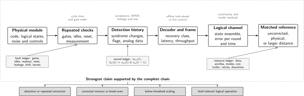
A QEC claim is an end-to-end comparison. Component faults enter a repeated check circuit; the measured history is converted into detection events; a declared decoder produces a recovery or Pauli-frame update; and the resulting logical channel is compared with a matched reference. Cycle time, leakage, decoder latency, state-preparation and measurement treatment, acceptance, and resource count remain part of the claim rather than disappearing behind the word “logical.”

Separate the evidence levels

Evidence level	What is established	What is not yet established
error detection	a fault changes one or more measured checks or flags	that the logical state was improved
repeated extraction	a syndrome history is acquired over several cycles	that decoding and recovery beat doing nothing
corrected logical memory	the decoded logical channel outperforms a named reference	scaling with code size or protected gates
below-threshold scaling	increasing distance suppresses a matched logical error metric	useful logical operations or practical overhead
fault-tolerant operation	a logical preparation, measurement, or gate limits fault propagation as specified	a universal, scalable computer
integrated architecture	multiple protected primitives compose with live control and resource management	arbitrarily deep useful computation

These levels form a partial order, not a marketing ladder. A small experiment can supply strong evidence for one level while intentionally leaving another untested. A repetition code may show clean distance scaling for bit flips while providing no protection against phase errors. A bosonic memory may beat every component in its module without demonstrating a family of increasing-distance codes. A surface-code memory may be below threshold while its logical gates, state factories, and decoder infrastructure remain above the required error budget.

Keep all resources inside the system boundary

The physical register is only part of a QEC machine. The accounting boundary should include, when used:

• data carriers, measurement ancillas, couplers, resonators, and reset modes;
• check gates, idle intervals, measurement, reset, leakage removal, and calibration;
• classical acquisition, decoding hardware, communication, and frame tracking;
• rejected shots, heralding, retries, dead time, and periodic retuning;
• extra modes or nonlinear elements used to encode and control a bosonic logical qubit.

This does not imply that every comparison must convert hardware into one universal scalar. It means that a favorable lifetime ratio must not silently exclude the ancilla whose failures dominate the syndrome path, or compare one logical cycle with one physical gate when their elapsed times differ by orders of magnitude.

A Worked Syndrome-Extraction Ledger

Ideal parity information

The three-qubit repetition code is a minimal laboratory for the distinction between a check value and a detection event. It encodes

$$|\psi\rangle = \alpha|0\rangle+\beta|1\rangle \quad\longmapsto\quad |\psi_L\rangle = \alpha|000\rangle+\beta|111\rangle$$

and uses the commuting $Z$-parity checks

$$S_1=Z_1Z_2, \qquad S_2=Z_2Z_3.$$

The complete one-bit-flip syndrome table is

Data operator	$S_1$	$S_2$	one-fault inference
$I$	$+1$	$+1$	no bit flip
$X_1$	$-1$	$+1$	flip qubit 1
$X_2$	$-1$	$-1$	flip qubit 2
$X_3$	$+1$	$-1$	flip qubit 3

The table is not a general decoder. It is valid for the declared candidate set $\{I,X_1,X_2,X_3\}$. Two data flips can mimic a different one-flip syndrome, and a phase error commutes with both checks. The code protects one classical axis of one logical qubit, not an arbitrary unknown qubit against arbitrary single-qubit noise.

An ancilla can measure $S_1$ by being prepared in $|0\rangle$, receiving controlled-NOT gates from data qubits 1 and 2, and then being measured in the computational basis. The result is the parity $q_1\mathbin{\oplus}q_2$ without revealing whether the data were $00$ or $11$. The same construction measures $S_2$. A physical implementation must additionally specify gate order, ancilla reset, crosstalk, leakage, and which ancilla faults can propagate back to the data.

Why repeated outcomes are not the decoder input

Let $m_j(t)\in\{+1,-1\}$ be the reported value of check $j$ in round $t$. Equivalently, define a measured syndrome bit

$$s_j(t) = \frac{1-m_j(t)}{2} \in\{0,1\}.$$

For a memory experiment, the useful local change is the detection event

$$\delta_j(t) = s_j(t)\mathbin{\oplus}s_j(t-1),$$

or, in the sign convention,

$$D_j(t) = m_j(t)m_j(t-1).$$

A value $D_j(t)=-1$ means that the reported parity changed across that time boundary. Suppose an $X_2$ data fault occurs between rounds $t-1$ and $t$. Both checks change, so the history contains simultaneous detection events at $(1,t)$ and $(2,t)$. By contrast, if only the reported value of check 1 is flipped in round $t$, then check 1 changes entering and leaving that bad sample. The likely pattern is two time-adjacent events at $(1,t)$ and $(1,t+1)$.

This spacetime distinction is the seed of surface-code decoding. It is also only a tendency. A gate fault can propagate to several data qubits; a leakage event can persist; correlated disturbances can create extended clusters; and the initial and final time boundaries can absorb an otherwise paired event. The Surface Code page develops the full decoding graph and boundary rules.

Detection, correction, and postselection

The same syndrome record can support three different protocols:

1. Detection with postselection. Reject every run containing specified events. Report both conditional logical quality and acceptance probability.
2. Offline correction. Preserve all declared runs, decode after the experiment, and reinterpret the final logical measurement.
3. Online correction or frame tracking. Decode during operation and apply a physical recovery or update a Pauli frame before a later noncommuting operation requires the result.

A Pauli frame avoids injecting unnecessary physical gates. If the decoder infers $X_2$, software records that future logical observables should be interpreted in the corresponding frame. Frame tracking is genuine correction when subsequent controls and final readout consume the frame consistently. It is not real-time correction merely because the final data analysis applies a sign after the run has ended.

Logical Metrics and Fair References

Characterize a channel, not one favorable state

An arbitrary logical qubit requires more than survival of $|0_L\rangle$. Let $\mathcal L_r$ denote the decoded logical channel after $r$ correction cycles. In a Pauli-transfer representation, a nearly Pauli-diagonal unital channel has

$$\mathsf R(\mathcal L_r) = \operatorname{diag} \left( 1, \lambda_X(r), \lambda_Y(r), \lambda_Z(r) \right).$$

The entanglement fidelity and average state fidelity are then

$$F_e(r) = \frac{ 1+\lambda_X(r)+\lambda_Y(r)+\lambda_Z(r) }{4},$$ $$F_{\rm avg}(r) = \frac12 + \frac{ \lambda_X(r)+\lambda_Y(r)+\lambda_Z(r) }{6}.$$

The two formulas have different normalizations and must not be interchanged. More importantly, three decay parameters reveal anisotropy that a single average can conceal. A repetition code can have excellent $\lambda_Z$-basis population survival while losing the conjugate logical coherence rapidly.

State preparation and measurement, usually abbreviated SPAM, require an explicit convention. One may jointly fit preparation, repeated-channel, and readout parameters; use reference sequences; or report raw end-to-end success. Subtracting SPAM is legitimate only when the fitted model and uncertainty remain visible. Raw and corrected quantities answer different questions.

From many rounds to an error per round

For a binary logical observable subject to independent identical flips with probability $\varepsilon_L$ per cycle, the odd-parity failure probability after $r$ cycles is

$$P_{\rm fail}(r) = \frac12 \left[ 1- \left(1-2\varepsilon_L\right)^r \right].$$

This exact relation is preferable to $P_{\rm fail}\approx r\varepsilon_L$ when the accumulated failure is not very small. Inverting it gives

$$\varepsilon_L = \frac12 \left[ 1- \left(1-2P_{\rm fail}(r)\right)^{1/r} \right].$$

The model assumes stationary, Markovian binary flips. A good fit does not prove those assumptions. Time-dependent calibration drift, burst events, and leakage can produce the same average curve while changing long-run risk. Residuals, time ordering, and event-cluster statistics therefore matter.

If one syndrome cycle lasts $\tau_{\rm cyc}$, a per-cycle error should also be translated into a time-normalized rate. For small $\varepsilon_L$,

$$\Gamma_L \simeq \frac{\varepsilon_L}{\tau_{\rm cyc}}.$$

Two implementations can have the same error per cycle while differing substantially in memory time because one cycle is much slower. Conversely, a fast cycle may tolerate a larger per-cycle error and still preserve a state longer in wall-clock time.

Break-even is a ratio with a named denominator

For a chosen lifetime convention, define the memory gain

$$G = \frac{\tau_L}{\tau_{\rm ref}}.$$

The reference might be:

• the best individual physical qubit available in the device;
• the median component qubit;
• the uncorrected encoded state using the same data degrees of freedom;
• the full encoded module with syndrome extraction disabled;
• an optimized direct physical memory using comparable elapsed time and control resources.

These denominators are scientifically useful but not equivalent. Beating an uncorrected encoding shows that the correction loop helps its own code. Beating the best component is a stronger module-level memory result. Neither alone demonstrates scalable distance suppression.

If $\tau_L$ and $\tau_{\rm ref}$ are independently estimated, a first-order uncertainty propagation is

$$\left( \frac{\sigma_G}{G} \right)^2 \simeq \left( \frac{\sigma_{\tau_L}}{\tau_L} \right)^2 + \left( \frac{\sigma_{\tau_{\rm ref}}}{\tau_{\rm ref}} \right)^2.$$

Shared calibration and model parameters create covariance and should be included rather than forced into this independent approximation. A central value $G>1$ is not convincing break-even evidence if the confidence interval substantially overlaps one.

Below threshold is a scaling statement

For a matched family of odd-distance topological memories under a fixed architecture, a common phenomenological form is

$$\varepsilon_d \propto \left( \frac{p}{p_{\rm th}} \right)^{(d+1)/2}.$$

The adjacent-distance suppression factor is

$$\Lambda_d = \frac{\varepsilon_d}{\varepsilon_{d+2}} \approx \frac{p_{\rm th}}{p}.$$

Thus $\Lambda_d>1$ means that the larger code performed better in the matched comparison. The approximate equality is not a device-independent law. Finite-size effects, biased noise, boundaries, leakage, correlations, decoder mismatch, and circuit changes can all make $\Lambda_d$ depend on $d$ and on the tested logical observable.

Three distinctions are essential:

• break-even: one corrected logical object beats one named reference;
• below threshold: a matched logical error decreases as code distance increases;
• fault-tolerant computation: preparations, measurements, gates, routing, decoding, and non-Clifford resources compose without losing the scaling advantage.

None of these phrases entails the next one automatically.

Case Study I: Repetition-Code Syndrome Histories

What the 2021 experiment tested

Google Quantum AI implemented cyclic bit- and phase-flip repetition codes on superconducting-qubit chains with up to 21 qubits, corresponding to code distance 11. Repeated stabilizer measurements generated a spacetime detection record over as many as 50 cycles. For the phase-flip repetition family, the reported logical error per round decreased from $8.7\times10^{-3}$ at five qubits to $6.7\times10^{-5}$ at 21 qubits. Fits gave suppression factors

$$\Lambda_X = 3.18\pm0.08, \qquad \Lambda_Z = 2.99\pm0.09.$$

The result established exponential suppression for the protected error type in these one-dimensional code families. It did not establish an arbitrary logical-qubit memory: each repetition experiment protected one Pauli sector while leaving its conjugate sector uncorrected.

The average detection-event fraction was about $11\%$ and remained stable across 50 rounds. That observation is operationally important. A low logical failure rate did not arise because the syndrome record was empty; the decoder regularly processed physical faults and measurement errors. The experiment also used the exact accumulated-failure relation above to distinguish an error per round from an end-of-experiment failure fraction.

Rare correlated events changed the evidence boundary

High-energy disturbances affected fewer than $0.5\%$ of experimental runs in the reported typical-behavior analysis, and those runs were removed. The choice was disclosed and scientifically useful for isolating the ordinary error process, but it changes the claim. The resulting suppression factor describes the accepted operating regime, not the unconditional long-duration service.

This is a general lesson. A rare event can be negligible in a short device benchmark yet dominate a target logical error rate of $10^{-9}$ or lower. Long-running QEC therefore needs both a typical-noise model and a tail-risk ledger:

$$P_{\rm fail} = P_{\rm typ}P_{\rm fail|typ} + P_{\rm burst}P_{\rm fail|burst}.$$

When $P_{\rm fail|burst}$ is near one, reducing $P_{\rm typ}$ by increasing distance eventually exposes the burst floor. Reporting the event rate, duration, spatial footprint, postselection rule, and recovery time is part of the QEC result.

Case Study II: Surface-Code Memory Scaling

Repeated extraction came before clear scaling

Early superconducting demonstrations established essential pieces in stages: repetitive parity detection, multi-round syndrome acquisition, decoder construction, and small surface-code patches. Krinner and collaborators realized repeated QEC in a distance-3 surface code in 2022. Such experiments are stronger than one-shot error detection because they exercise resets, measurement errors, temporal boundaries, and a decoder over several cycles. At distance 3, however, finite-size behavior and component overhead can still prevent the corrected logical memory from outperforming simpler references.

This staged progression should be described accurately. A repeated distance-3 circuit can validate extraction and decoding even when its logical lifetime is below break-even. Calling it useless would discard real engineering evidence; calling it scalable QEC would exceed the data.

Distance 5 versus distance 3 in 2023

In the 2023 surface-code scaling experiment, a 49-qubit distance-5 logical memory on a 72-qubit superconducting device was compared with an ensemble of distance-3 patches under a matched circuit. Over 25 cycles, the reported logical error per cycle was

$$\varepsilon_5 = (2.914\pm0.016)\%,$$

versus an average

$$\overline{\varepsilon}_3 = (3.028\pm0.023)\%.$$

The larger code was modestly better. That was an important finite-size crossing, but the ratio was close to one and far from the suppression needed for useful deep computation. The same study used repetition codes up to distance 25 to expose a floor associated with rare high-energy events. The surface-code and repetition-code results therefore supplied complementary evidence: broader quantum protection at small distance and stronger diagnostics of correlated tails in a simpler geometry.

Distance 7 below threshold in 2025

The Willow experiment compared distance-5 and distance-7 surface-code memories. Its distance-7 implementation used 101 qubits: 49 data qubits, 48 measurement qubits, and four leakage-removal qubits. The reported distance-7 logical error per cycle was

$$\varepsilon_7 = (0.143\pm0.003)\%,$$

with a distance-step suppression factor

$$\Lambda = 2.14\pm0.02.$$

The distance-7 logical lifetime was $291\pm6\ \mu{\rm s}$. The constituent physical qubits had a median lifetime of $85\pm7\ \mu{\rm s}$ and a best reported lifetime of $119\pm13\ \mu{\rm s}$, giving a gain of $2.4\pm0.3$ over that best physical reference. This combined two distinct claims: increasing distance suppressed the matched logical error, and the distance-7 logical memory outlived the declared component reference.

Classical control was part of the experiment. A real-time distance-5 decoder had an average latency of $63\ \mu{\rm s}$ while syndrome cycles arrived every $1.1\ \mu{\rm s}$, and the system was exercised for up to one million cycles. Latency longer than one cycle is not automatically fatal if decoding is pipelined and the backlog remains bounded. What matters is throughput, tail latency, memory growth, and whether later operations receive the frame before they depend on it.

Long repetition-code runs on the same platform found rare correlated events roughly once per hour, or once per approximately $3\times10^9$ cycles, producing a projected logical floor near $10^{-10}$ for that diagnostic. This does not erase the below-threshold result. It states where the simple independent-fault scaling law is expected to stop without additional mitigation.

Most importantly, the experiment was a logical memory result. It did not by itself demonstrate a universal set of below-threshold logical gates, magic-state production, large-scale routing, or a useful fault-tolerant algorithm. The source itself identifies those as remaining challenges.

Case Study III: What Logical Lifetime Should Beat

A reference ladder

A lifetime headline becomes interpretable when placed in a reference ladder:

Reference	Question answered when the logical memory wins
same encoding, correction disabled	does the correction loop help this encoding?
best physical component in the module	is the complete encoded memory better than every constituent memory?
median physical component	does redundancy beat a typical component?
optimized standalone physical qubit	does encoding beat the strongest available direct memory under a declared resource boundary?
larger-distance logical memory	is there scalable suppression rather than one favorable crossing?

No row makes the others redundant. The uncorrected encoding can be a poor baseline because it contains extra lossy levels or more carriers without using their syndrome information. The best physical component can fluctuate because of device selection. A larger-distance comparison can show scaling while every tested logical lifetime remains shorter than a physical qubit.

A fair comparison aligns:

• the initial logical-state ensemble and measured observables;
• elapsed storage time rather than cycle count alone;
• whether SPAM is included or removed;
• active control, echo pulses, and refresh operations;
• acceptance probability and excluded records;
• uncertainty and device-selection procedure.

If the logical memory is tested only on $|0_L\rangle$ while the physical reference is averaged over six cardinal states, the ratio mixes state dependence with correction. If the logical experiment receives continuous active feedback while the physical reference is left idle despite having an available echo sequence, the comparison measures a protocol choice as well as an encoding.

Memory gain is not gate gain

A protected idle channel can tolerate a syndrome pipeline that finishes after the measured interval. A logical gate must also limit fault propagation, maintain code distance through deformation or teleportation, and deliver its frame before dependent operations. Its natural metric is an operation error or process fidelity, not the memory lifetime ratio.

Likewise, a decoder can improve a final measurement offline without demonstrating low-latency control. Offline decoding is excellent evidence for the code and noise model. Online decoding is additional systems evidence. Both should be reported, and neither should be relabeled as the other.

Case Study IV: Bosonic Logical Memories

One oscillator is a module, not one physical level

Bosonic codes store redundancy in the many levels of an oscillator. Cat and binomial codes often diagnose photon loss through parity-like information; Gottesman–Kitaev–Preskill codes diagnose small phase-space displacements through modular quadratures. Their physical-resource ledger can include a high-quality storage mode, a nonlinear ancilla, readout resonators, pumps, reset channels, and real-time controllers.

That architecture changes the comparison, not the standard of evidence. A bosonic QEC experiment should still report:

1. the finite-energy code states actually prepared;
2. the dominant oscillator, ancilla, and control errors;
3. the syndrome observable and extraction cadence;
4. whether correction is active, autonomous, or applied in a frame;
5. the full logical-state ensemble;
6. the uncorrected and physical references;
7. accepted runs, restarts, and feedback latency.

The Bosonic Qubits page develops hardware requirements and the broader evidence timeline. Cat Codes owns the coherent-component encoding, parity-sector recovery, and distinction between loss-correcting cats and biased stabilized cat qubits. The three cases below illustrate how the benchmark denominator changed.

Cat-code process lifetime in 2016

Ofek and collaborators repeatedly monitored photon-number parity in a superconducting cavity encoding. The parity history located likely single-photon-loss events, and the experiment tracked the associated logical phase. The corrected process lifetime was approximately $320\ \mu{\rm s}$, about $2.2$ times the uncorrected encoded lifetime and about $1.1$ times the best physical reference used in the comparison.

The two ratios answer different questions. The larger ratio showed that syndrome tracking substantially improved the selected encoding. The smaller ratio showed a modest crossing of the stronger component benchmark. The experiment did not supply an increasing-distance threshold curve; it supplied an end-to-end logical-memory comparison in one oscillator module.

GKP beyond break-even in 2023

Sivak and collaborators implemented repeated real-time correction of a finite-energy GKP qubit in a superconducting oscillator. The protocol used an ancilla-assisted correction cycle optimized with reinforcement learning and stabilized the logical state continuously. The reported coherence gain over the imperfect components of the module was

$$G_{\rm GKP} = 2.27\pm0.07.$$

This is strong beyond-break-even memory evidence because the denominator included the available imperfect components rather than only the uncorrected GKP encoding. It remains a memory result for one encoded oscillator. Scaling evidence would require a declared family, additional distance or concatenation parameter, and matched logical-error comparisons.

Discrete-variable binomial encoding in 2023

Binomial Codes derives the finite-superposition family and its modular-number recovery. In the 2023 experiment, Ni and collaborators encoded a qubit in selected photon-number states of a microwave cavity. A frequency-comb control pulse repeatedly extracted the error syndrome, and feedback corrected the inferred error. The resulting logical lifetime exceeded the best physical reference by approximately $16\%$.

A $16\%$ crossing and a factor-of-two crossing are both break-even results when their uncertainties and denominators support $G>1$; the factors should not be ranked without comparing state ensemble, lifetime definition, module boundary, cycle duration, and hardware generation. The binomial and GKP experiments also target different correctable-error structures. Their value lies in demonstrating two routes to a complete correction loop, not in declaring one universal winner.

What a bosonic break-even result does not imply

Bosonic modules can reduce the number of separately addressable physical elements needed for one logical qubit, but they do not remove overhead. Finite-energy codewords, ancilla-induced errors, nonlinear control, oscillator leakage, and repeated reset all remain. Concatenating a bosonic inner code with an outer qubit code may yield scalable suppression, but then both layers, their interfaces, and their correlated failure modes belong in the evidence contract.

From Memories to Fault-Tolerant Architectures

A current neutral-atom experiment provides a useful contrast between a memory benchmark and a broader architecture demonstration. Bluvstein and collaborators used reconfigurable arrays of up to 448 atoms and repeated surface-code QEC. In a four-round characterization, the distance-5 code had $2.14(13)$ times lower error per round than distance 3. Loss information and machine-learning decoding improved the QEC result by $1.73(13)$ times. The same platform demonstrated ingredients including transversal logical operations, lattice surgery, teleportation between codes, qubit reset, and constant-entropy operation.

The strongest accurate label is fault-tolerant architecture building blocks with below-threshold memory evidence. The result integrates more logical operations than an idle-memory experiment, but four rounds and a catalog of primitives are not an arbitrarily deep useful computation. The claim must preserve both facts: the architecture evidence is substantial, and system-scale algorithmic fault tolerance remains a further integration test.

This distinction becomes increasingly important as experiments combine several individually impressive ingredients. “All ingredients demonstrated” means that each named mechanism appeared under the stated conditions. It does not prove that the full stack has already been composed at the target logical error, throughput, and resource overhead.

Evidence Ladder

Level 1: syndrome sensitivity

Checks respond to injected or naturally occurring faults with the expected pattern. This validates observability and calibration, not logical improvement.

Level 2: repeated detection and a decoder

Noisy check outcomes are collected across time, temporal boundaries are closed, and a declared decoder predicts final logical outcomes. Acceptance and offline information remain visible.

Level 3: logical improvement

The complete corrected channel beats an uncorrected encoding or physical reference with uncertainty. The protected state ensemble and system boundary are declared.

Level 4: matched scaling

Increasing distance or another protection parameter suppresses logical error under a fixed architecture contract. Multiple sizes and both logical sectors are preferable to one pair and one basis.

Level 5: fault-tolerant logical operations

Encoded preparations, measurements, and gates retain the intended scaling, with decoder and frame latency compatible with composition.

Level 6: sustained integrated computation

The system repeatedly prepares resources, corrects memories and operations, routes logical information, manages leakage and entropy, and completes a declared workload with an auditable resource advantage.

Common Mistakes

• Equating a nonzero syndrome with successful correction.
• Calling a repetition-code result arbitrary-qubit QEC.
• Quoting final failure probability as error per round without a model.
• Comparing errors per cycle when cycle durations differ substantially.
• Using an uncorrected encoding as though it were the only possible physical reference.
• Removing burst events without reporting their frequency and the resulting conditional claim.
• Calling $\Lambda>1$ at one size pair a universal threshold number.
• Treating a longer logical memory as evidence for fault-tolerant gates.
• Omitting ancillas, extra modes, reset hardware, or classical decoding from a bosonic or stabilizer-code resource boundary.
• Calling offline relabeling real-time feedback.
• Reporting only the best logical basis or best device instance.
• Extrapolating an independent-fault power law below an observed correlated error floor.

Reporting Checklist

1. State the code family, distance or protection parameter, logical operators, and tested logical-state ensemble.
2. Give the complete check circuit, gate order, cycle time, reset procedure, and initial and final time-boundary conventions.
3. Report physical gate, idle, measurement, reset, loss, leakage, and correlation diagnostics relevant to the circuit.
4. Define syndrome bits, detection events, analog side information, and any event flags supplied to the decoder.
5. Identify the decoder version, training data, priors, offline look-ahead, throughput, mean and tail latency, and frame-consumption point.
6. Distinguish postselection, final-readout correction, Pauli-frame tracking, physical feedback, and autonomous correction.
7. Define the logical metric, SPAM treatment, fit model, confidence interval, and residual or goodness-of-fit checks.
8. Report both per-cycle and per-time quantities.
9. Name every break-even denominator and align state ensemble, elapsed time, and active controls.
10. For threshold claims, hold the architecture contract fixed across distances and report both logical sectors when applicable.
11. Preserve chronological data long enough to reveal drift, bursts, leakage persistence, and correlated event clusters.
12. Report accepted shots, rejected shots, reason codes, retries, downtime, calibration cadence, and unconditional delivery probability.
13. Count data carriers, ancillas, couplers, oscillator modes, readout and reset resources, and classical hardware inside the chosen boundary.
14. State exactly which evidence label is supported and which next integration step remains untested.

Exercises

1. Decode the bit-flip syndrome

For the three-qubit repetition code with $S_1=Z_1Z_2$ and $S_2=Z_2Z_3$, a round returns $(m_1,m_2)=(-1,+1)$. Under the one-bit-flip candidate set, infer the error. Why is that inference not valid under unrestricted two-qubit faults?

Solution

The syndrome table assigns $(-1,+1)$ to $X_1$, so the one-fault decoder chooses $X_1$ as the recovery or updates the corresponding frame.

Under unrestricted two-qubit faults, $X_2X_3$ has the same syndrome: $X_2X_3$ anticommutes with $S_1$ once and with $S_2$ twice. The syndrome therefore identifies an equivalence class only relative to the assumed error set. Applying an $X_1$ recovery after $X_2X_3$ leaves $X_1X_2X_3=\overline X$, a logical error.

2. Distinguish data and measurement faults

One check reports the sign sequence

$$\left( m(t-1),m(t),m(t+1),m(t+2) \right) = \left( +1,-1,+1,+1 \right).$$

Locate the detection events and give the simplest measurement-fault explanation. How would a persistent data fault differ?

Solution

The detection products are

$$D(t)=-1, \qquad D(t+1)=-1, \qquad D(t+2)=+1.$$

There are two adjacent-time detection events at the same check. The simplest explanation is one incorrect check measurement in round $t$.

A persistent data fault that changes this check between $t-1$ and $t$ would usually leave the true check sign at $-1$ until a later recovery or second fault. It therefore creates an event at the onset and another only when the parity changes back, not necessarily in the immediately following round.

3. Infer an error per round

A binary logical observable fails with probability $P_{\rm fail}=0.18$ after $r=20$ cycles. Under the independent identical-flip model, estimate $\varepsilon_L$. Compare it with the small-error estimate $P_{\rm fail}/r$.

Solution

The exact inversion gives

$$\varepsilon_L = \frac12 \left[ 1- \left(1-0.36\right)^{1/20} \right] \approx 0.0110.$$

The linear estimate is

$$\frac{0.18}{20}=0.009.$$

The linear approximation underestimates the per-cycle flip probability because multiple flips can cancel in the final parity. At smaller accumulated failure, the two estimates converge.

4. Per cycle versus per time

Memory A has $\varepsilon_A=1.2\times10^{-3}$ per $1.0\ \mu{\rm s}$ cycle. Memory B has $\varepsilon_B=7.0\times10^{-4}$ per $2.5\ \mu{\rm s}$ cycle. Which is better per cycle and which has the smaller small-error rate per unit time?

Solution

Memory B has the smaller error per cycle. The approximate time-normalized rates are

$$\Gamma_A \simeq 1.2\times10^3\ {\rm s}^{-1},$$ $$\Gamma_B \simeq \frac{7.0\times10^{-4}} {2.5\times10^{-6}\ {\rm s}} = 2.8\times10^2\ {\rm s}^{-1}.$$

Memory B is also better per unit time in this example. The calculation shows why both quantities must be reported; the per-cycle ranking alone does not guarantee the per-time ranking.

5. Interpret a suppression factor

A matched code family has $\varepsilon_3=8.0\times10^{-3}$ and $\varepsilon_5=3.2\times10^{-3}$. Compute $\Lambda_3$. If the same factor continued, project $\varepsilon_7$. Give two reasons not to present the projection as a measured result.

Solution

The measured adjacent-distance factor is

$$\Lambda_3 = \frac{\varepsilon_3}{\varepsilon_5} = 2.5.$$

Naive continuation gives

$$\varepsilon_7 \approx \frac{\varepsilon_5}{2.5} = 1.28\times10^{-3}.$$

This is an extrapolation. Finite-size effects can make $\Lambda_d$ depend on distance, and leakage or correlated bursts can produce a floor. Decoder and circuit changes at the next size can also invalidate the matched-family assumption.

6. Test a break-even claim

A logical lifetime is $\tau_L=230\pm8\ \mu{\rm s}$ and the chosen reference is $\tau_{\rm ref}=205\pm7\ \mu{\rm s}$. Assuming independent uncertainties, estimate $G$ and $\sigma_G$. Is “beyond break-even” a well-supported concise label?

Solution

The gain is

$$G = \frac{230}{205} \approx 1.122.$$

Independent propagation gives

$$\sigma_G \approx G \sqrt{ \left(\frac{8}{230}\right)^2 + \left(\frac{7}{205}\right)^2 } \approx 0.055.$$

Thus $G\approx1.12\pm0.06$. The central value exceeds one by a little more than two standard uncertainties. “Beyond break-even against the stated reference” is defensible if the fit model, covariance, and state ensemble are sound, but the modest margin and exact denominator should remain visible.

7. Choose a bosonic reference

A corrected oscillator code outlives the same encoding with correction disabled by a factor of $3.0$, but reaches only $0.9$ times the lifetime of the nonlinear ancilla used for syndrome extraction. What claims are supported?

Solution

The experiment supports correction improves the encoded memory by a factor of three relative to its uncorrected version. It does not support beyond the best component under the stated module boundary, because the logical lifetime is shorter than the ancilla lifetime.

Both facts are useful. The first diagnoses an effective correction loop; the second shows that the stronger module-level break-even target has not yet been crossed. Neither ratio alone establishes distance scaling or fault-tolerant logical gates.

8. Classify the evidence

An experiment runs distance-3 and distance-5 surface-code memories for four rounds. Distance 5 has half the logical failure probability. The same device demonstrates a logical entangling primitive in a separate circuit, but no combined long computation. Assign the strongest justified labels.

Solution

The matched distance comparison supports finite-distance below-threshold memory evidence for the tested four-round protocol, assuming the circuit, decoder, and metric are genuinely matched. The separate logical primitive supports a demonstrated fault-tolerant architecture building block if its fault-propagation conditions were verified.

The evidence does not yet establish sustained universal fault-tolerant computation. The memory scaling and logical primitive were not composed into an arbitrarily deep workload, and four rounds do not characterize long-time drift, decoder backlog, or rare-event floors.

References

1. E. Knill and R. Laflamme, “Theory of quantum error-correcting codes,” Physical Review A 55, 900–911 (1997), doi:10.1103/PhysRevA.55.900.
2. D. Gottesman, “Stabilizer codes and quantum error correction,” PhD thesis, California Institute of Technology (1997), arXiv:quant-ph/9705052.
3. E. Dennis, A. Kitaev, A. Landahl, and J. Preskill, “Topological quantum memory,” Journal of Mathematical Physics 43, 4452–4505 (2002), doi:10.1063/1.1499754.
4. A. G. Fowler, M. Mariantoni, J. M. Martinis, and A. N. Cleland, “Surface codes: Towards practical large-scale quantum computation,” Physical Review A 86, 032324 (2012), doi:10.1103/PhysRevA.86.032324.
5. B. M. Terhal, “Quantum error correction for quantum memories,” Reviews of Modern Physics 87, 307–346 (2015), doi:10.1103/RevModPhys.87.307.
6. J. Kelly et al., “State preservation by repetitive error detection in a superconducting quantum circuit,” Nature 519, 66–69 (2015), doi:10.1038/nature14270.
7. A. D. Córcoles et al., “Demonstration of a quantum error detection code using a square lattice of four superconducting qubits,” Nature Communications 6, 6979 (2015), doi:10.1038/ncomms7979.
8. Google Quantum AI, “Exponential suppression of bit or phase errors with cyclic error correction,” Nature 595, 383–387 (2021), doi:10.1038/s41586-021-03588-y.
9. C. Ryan-Anderson et al., “Realization of real-time fault-tolerant quantum error correction,” Physical Review X 11, 041058 (2021), doi:10.1103/PhysRevX.11.041058.
10. L. Egan et al., “Fault-tolerant control of an error-corrected qubit,” Nature 598, 281–286 (2021), doi:10.1038/s41586-021-03928-y.
11. S. Krinner et al., “Realizing repeated quantum error correction in a distance-three surface code,” Nature 605, 669–674 (2022), doi:10.1038/s41586-022-04566-8.
12. Google Quantum AI, “Suppressing quantum errors by scaling a surface code logical qubit,” Nature 614, 676–681 (2023), doi:10.1038/s41586-022-05434-1.
13. Google Quantum AI and Collaborators, “Quantum error correction below the surface code threshold,” Nature 638, 920–926 (2025), doi:10.1038/s41586-024-08449-y.
14. D. Bluvstein et al., “A fault-tolerant neutral-atom architecture for universal quantum computation,” Nature 649, 39–46 (2026), doi:10.1038/s41586-025-09848-5.
15. D. A. Lidar and T. A. Brun, editors, Quantum Error Correction, Cambridge University Press (2013), doi:10.1017/CBO9781139034807.
16. D. Litinski, “A game of surface codes: Large-scale quantum computing with lattice surgery,” Quantum 3, 128 (2019), doi:10.22331/q-2019-03-05-128.
17. O. Higgott and C. Gidney, “Sparse blossom: Correcting a million errors per core second with minimum-weight matching,” Quantum 9, 1600 (2025), doi:10.22331/q-2025-01-20-1600.
18. D. Gottesman, A. Kitaev, and J. Preskill, “Encoding a qubit in an oscillator,” Physical Review A 64, 012310 (2001), doi:10.1103/PhysRevA.64.012310.
19. M. H. Michael et al., “New class of quantum error-correcting codes for a bosonic mode,” Physical Review X 6, 031006 (2016), doi:10.1103/PhysRevX.6.031006.
20. N. Ofek et al., “Extending the lifetime of a quantum bit with error correction in superconducting circuits,” Nature 536, 441–445 (2016), doi:10.1038/nature18949.
21. L. Hu et al., “Quantum error correction and universal gate set operation on a binomial bosonic logical qubit,” Nature Physics 15, 503–508 (2019), doi:10.1038/s41567-018-0414-3.
22. P. Campagne-Ibarcq et al., “Quantum error correction of a qubit encoded in grid states of an oscillator,” Nature 584, 368–372 (2020), doi:10.1038/s41586-020-2603-3.
23. J. M. Gertler et al., “Protecting a bosonic qubit with autonomous quantum error correction,” Nature 590, 243–248 (2021), doi:10.1038/s41586-021-03257-0.
24. V. V. Sivak et al., “Real-time quantum error correction beyond break-even,” Nature 616, 50–55 (2023), doi:10.1038/s41586-023-05782-6.
25. Z. Ni et al., “Beating the break-even point with a discrete-variable-encoded logical qubit,” Nature 616, 56–60 (2023), doi:10.1038/s41586-023-05784-4.
26. H. Putterman et al., “Hardware-efficient quantum error correction via concatenated bosonic qubits,” Nature 638, 927–934 (2025), doi:10.1038/s41586-025-08642-7.

Further Connections

• Logical Benchmarking defines the reusable protocol contract behind logical channels, suppression factors, break-even, protected-gate tests, and delivered performance.
• Threshold Theorem separates a rigorous sufficient bound, an asymptotic critical point, a finite-size crossing, a pseudothreshold, and experimental scaling evidence.
• Magic State Distillation separates logical preparation, a bounded accepted distillation block, and an algorithm-scale factory service, with the evidence through August 2026.
• Common Noise Models distinguishes stochastic Pauli approximations from leakage, drift, coherent, and correlated noise.
• Metrics for Quantum Hardware defines coherence, logical channels, leakage, and workload-level metrics.
• Reporting Standards gives the volume-wide artifact and uncertainty requirements.
• Claims, Hype, and Evidence Standards supplies the general claim-audit framework.
• Negative Results and Limitations scopes structural code bounds, mitigation overheads, and claims that remain open at larger scale.
• Quantum Information Roadmap places QEC after channels, composite systems, gates, and classical decoding prerequisites.