Sensing Case Studies

Short Definition

A sensing case study follows a physical quantity from its operational definition through quantum transduction, control, readout, estimation, calibration, nuisance-parameter correction, and validation. The result is not merely a narrow resonance, a large quantum Fisher information, or the smallest resolvable signal in one trace. It is an estimate or detection claim with a declared bandwidth, averaging time, spatial support, resource denominator, and uncertainty statement.

This page compares five implementations:

• a Ramsey-interrogated atomic clock;
• optical clocks using spin-squeezed ensembles;
• nitrogen-vacancy-center magnetometry;
• a transportable atom-interferometric gravimeter;
• Rydberg-atom microwave electrometry.

Quantum Measurement as Estimation owns the general likelihood, estimator, loss, uncertainty, and validation framework. Classical and Quantum Fisher Information owns the detector-dependent and measurement-optimized local information metrics. Standard Quantum Limit owns independent-probe scaling and resource caveats. Heisenberg Scaling owns the ideal inverse-resource law, global phase caveats, and noisy asymptotic limits. Squeezing owns the cross-platform relation among reduced fluctuations, signal response, readout, loss, and a defensible metrological-gain claim. The detailed clock, defect, atom-optics, and Rydberg physics live in their respective canonical pages. This page owns the end-to-end comparison of sensing evidence.

The Metrology Contract

Define the measurand

The same instrument can be described as measuring a field amplitude, one Cartesian component, a frequency, a phase, a gradient, a power spectral density, or a model coefficient. Those are different estimands. Write the measurement model before quoting a sensitivity:

$$D \sim p \left( D \mid \theta, \boldsymbol\nu, \mathcal C \right).$$

Here $D$ is the acquired record, $\theta$ the measurand, $\boldsymbol\nu$ nuisance parameters, and $\mathcal C$ the preparation, control, readout, calibration, and selection protocol. The reported estimator is

$$\widehat\theta = \mathcal A(D;\mathcal C),$$

and its interpretation requires both random uncertainty and possible bias:

$$b(\theta) = \mathbb E_\theta[\widehat\theta]-\theta.$$

A local Cramér–Rao bound or quantum Fisher information can identify an ideal variance floor. It does not by itself establish that the estimator is unbiased, the nuisance model is correct, confidence intervals cover, or the sensor is calibrated to the external quantity of interest.

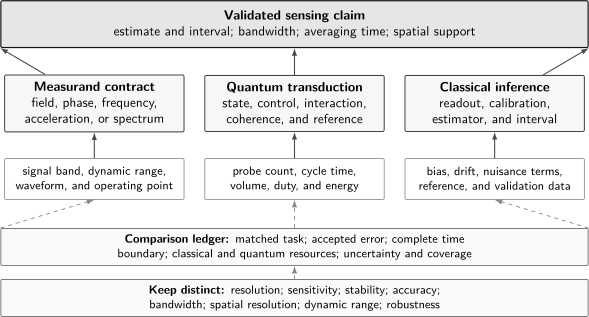
A sensing claim is end to end only when the measurand, signal band, quantum transducer, cycle resources, estimator, nuisance model, reference, and uncertainty survive the same audit. Sensitivity, stability, accuracy, resolution, bandwidth, spatial resolution, and dynamic range are not synonyms.

Keep the performance labels separate

Label	Operational question
resolution	What signal increment can the readout digitization or fitted model distinguish under stated conditions?
sensitivity	How much random uncertainty is obtained per square root bandwidth or averaging resource?
stability	How does the measured output fluctuate with averaging time or lag?
accuracy	How closely does the corrected estimate track the defined measurand, including bias uncertainty?
bandwidth	Over which frequencies does the response and calibration apply?
dynamic range	Over what input range is the inverse model unique and acceptably linear?
spatial resolution	Over what sensing volume or point-spread function is the quantity averaged?
robustness	How does performance change with environment, alignment, aging, and operator intervention?

For white, independent measurement noise, a commonly quoted amplitude sensitivity is

$$\eta_\theta \equiv \delta\theta \sqrt{T_{\mathrm{avg}}},$$

with units such as $\mathrm{T}/\sqrt{\mathrm{Hz}}$ or $\mathrm{m\,s^{-2}}/\sqrt{\mathrm{Hz}}$. This shorthand is not valid across arbitrary averaging times. Drift, $1/f$ noise, dead-time aliasing, correlated samples, estimator nonlinearity, and bandwidth conventions can all break the $T_{\mathrm{avg}}^{-1/2}$ law.

For clocks, Allan deviation $\sigma_y(\tau)$ is a stability statistic for fractional frequency $y$. For field sensors, an amplitude spectral density or a filter-weighted uncertainty may be more natural. A paper should state whether a spectrum is one-sided or two-sided and whether a quoted bandwidth is equivalent noise bandwidth, control bandwidth, or the range over which calibration was tested.

Count the complete cycle

A pulsed sensor has cycle time

$$\begin{aligned} T_c ={}& T_{\mathrm{prepare}} + T_{\mathrm{interrogate}} \\ &+ T_{\mathrm{read}} + T_{\mathrm{reset}} + T_{\mathrm{dead}}. \end{aligned}$$

The duty factor is

$$d = \frac{ T_{\mathrm{interrogate}} }{ T_c }.$$

Longer interrogation usually increases phase response but can reduce contrast, narrow unambiguous range, expose drift, and lengthen the cycle. The resource contract should include probe number, interrogation time, number of cycles, sensor volume, bandwidth, local oscillator, auxiliary classical sensors, control power, calibration time, rejected data, and postprocessing.

Case Study 1: A Ramsey Atomic Clock

Quantum phase becomes a clock error signal

An ideal Ramsey sequence prepares a superposition, lets it accumulate phase for time $T$, and converts phase into excited-state population. A useful fringe model is

$$P_e(\nu) = P_0 + \frac{C}{2} \cos \left[ 2\pi(\nu-\nu_0)T+\phi_c \right],$$

where $\nu$ is the local-oscillator frequency, $\nu_0$ the unperturbed clock transition, $C$ the contrast, and $\phi_c$ a controlled phase. The clock samples opposite sides of the fringe to form an error signal and steers the local oscillator. The useful output is the disciplined oscillator, not the atomic population itself.

At mid-fringe, $N$ independent atoms with projection noise $\Delta P_e\simeq1/(2\sqrt N)$ give an ideal single-cycle fractional frequency uncertainty

$$\delta y_{\mathrm{QPN}} \simeq \frac{ 1 }{ 2\pi\nu_0TC\sqrt N }.$$

For uncorrelated cycles, the corresponding clock contribution scales as

$$\sigma_y^{\mathrm{QPN}}(\tau) \simeq \frac{ 1 }{ 2\pi\nu_0TC\sqrt N } \sqrt{ \frac{T_c}{\tau} }.$$

This expression exposes several levers: increase carrier frequency, interrogation time, contrast, atom number, or duty factor. It is not a complete clock budget. Local-oscillator phase noise, finite pulse duration, detection noise, collisions, Zeeman and Stark shifts, blackbody radiation, microwave-cavity phase, gravitational potential, and servo error can dominate different timescales.

Dead time is particularly important. Periodic sampling aliases local- oscillator noise near harmonics of the cycle frequency into the clock output, producing the Dick effect. More atoms cannot remove that aliasing. Zero-dead- time or interleaved ensembles, improved local oscillators, and sensitivity- function engineering attack a different resource than projection noise.

Ramsey Interferometry owns the pulse sequence, finite-pulse line shape, phase conventions, and error-signal derivation. Atomic Clocks owns the servo, stability, systematic uncertainty, time scale, and SI architecture.

NIST-F2 as a system case

The first accuracy evaluation of the NIST-F2 caesium fountain illustrates why a clock is more than its fringe. Laser-cooled caesium atoms traversed a Ramsey microwave cavity on the upward and downward portions of their ballistic flight. The interrogation region was held near $80\ \mathrm K$, reducing blackbody-radiation-shift uncertainty by more than a factor of 50 relative to the warmer architecture discussed by the authors. The cavity quality factor exceeded approximately $50{,}000$.

For the 2013 evaluation reported in 2014, the type-B fractional uncertainty was $0.11\times10^{-15}$ and the statistical type-A contribution was $0.44\times10^{-15}$. The labels matter:

• the type-A term characterized finite statistical evaluation against the comparison system;
• the type-B budget combined evaluated systematic effects and their uncertainties;
• neither number was simply the one-shot quantum projection limit;
• reducing blackbody uncertainty did not eliminate microwave-amplitude, cavity-phase, Zeeman, collision, Doppler, or gravitational corrections.

This is an accuracy-evaluation case, not a claim that one clock output was known absolutely without a comparison chain. It demonstrates how a quantum transition, cryogenic environment, microwave engineering, maser flywheel, servo, and uncertainty budget jointly realize a primary frequency standard.

Case Study 2: Spin-Squeezed Optical Clocks

The useful squeezing parameter

For $N$ effective two-level atoms, define collective spin

$$J_k = \frac12 \sum_{i=1}^{N} \sigma_k^{(i)}.$$

A coherent spin state polarized along $x$ has $\lvert\langle\mathbf J\rangle\rvert\simeq N/2$ and transverse variance $N/4$. The Wineland metrological squeezing parameter is

$$\xi_R^2 = \frac{ N (\Delta J_\perp)^2 }{ \lvert \langle\mathbf J\rangle \rvert^2 }.$$

When $\xi_R^2<1$, the state improves small-phase estimation over the matched coherent spin state and certifies useful multipartite entanglement under the usual collective-spin conditions. The ideal phase uncertainty becomes

$$\delta\phi \simeq \frac{\xi_R}{\sqrt N},$$

and the metrological gain in decibels is

$$G_{\mathrm{dB}} = -10\log_{10}\xi_R^2.$$

Noise reduction alone is insufficient. A strong quantum-nondemolition measurement or interaction can shrink $(\Delta J_\perp)^2$ while also shortening the mean spin, reducing contrast, losing atoms, adding phase noise, or increasing cycle time. The Wineland denominator correctly charges loss of coherence, but an end-to-end clock must additionally charge squeezing preparation, readout, dead time, local-oscillator noise, and technical fluctuations.

In a projection-noise-limited Ramsey clock, replacing a coherent state by a squeezed state suggests

$$\sigma_y^{\mathrm{sq}}(\tau) \simeq \xi_R \sigma_y^{\mathrm{QPN}}(\tau).$$

The relation holds only when the clock operates in the small-phase range and other noise remains below the squeezed projection noise. A state with $10\ \mathrm{dB}$ spectroscopic squeezing need not improve a running clock by $10\ \mathrm{dB}$.

Two direct clock comparisons

Eckner and collaborators used Rydberg interactions in a programmable strontium tweezer clock to generate almost $4\ \mathrm{dB}$ of metrological gain. In a synchronous comparison of independent squeezed states they reported fractional-frequency stability

$$\sigma_y(1\ \mathrm s) = 1.087(1)\times10^{-15},$$

$1.94(1)\ \mathrm{dB}$ below the standard quantum limit under the paper’s matched comparison. The differential measurement reached fractional precision at the $10^{-17}$ level in about half an hour. Synchronous interrogation rejected common local-oscillator noise, making the atomic quantum-noise comparison visible.

Robinson and collaborators used cavity quantum electrodynamics and quantum-nondemolition measurements to squeeze two independently addressable optical-clock subensembles. Their differential clock data directly showed a $1.9(2)\ \mathrm{dB}$ stability enhancement at the $10^{-17}$ level without subtracting technical noise. The absolute comparison nevertheless remained above the paper’s effective standard quantum limit because residual technical noise still contributed.

Together the results establish something stronger than inferred squeezing: entanglement improved measured clock comparisons after state preparation and readout. They do not establish universal Heisenberg scaling, a lower systematic uncertainty, or the same gain in an asynchronous clock network. A mature comparison should report the coherent-state reference, atom loss, contrast, cycle time, phase range, local-oscillator correlation, technical noise, and whether any noise was subtracted.

Case Study 3: NV-Center Magnetometry

A solid-state spin transducer

The negatively charged nitrogen-vacancy center in diamond has an electronic spin-triplet ground state, optical initialization and fluorescence readout, and coherent microwave control at room temperature. A common effective model is

$$\frac{H}{\hbar} = DS_z^2 + \gamma_e \mathbf B\mathbin{\cdot}\mathbf S + E(S_x^2-S_y^2) + H_{\mathrm{hf}} + H_{\mathrm{strain}}.$$

The zero-field splitting $D$, electron gyromagnetic ratio $\gamma_e$, transverse strain parameter $E$, hyperfine coupling, and crystal-axis orientation all enter the inverse problem. Near an NV axis, the two $m_s=0\leftrightarrow m_s=\pm1$ resonance frequencies shift approximately as

$$\omega_\pm \simeq D \pm \gamma_e B_\parallel.$$

This supports continuous-wave resonance magnetometry, pulsed Ramsey sensing, echo-based ac magnetometry, relaxometry, and correlation spectroscopy. NV Centers and Solid-State Defects owns the level structure, optical pumping, readout, relaxation, dephasing, and open-system interpretation.

For a pulsed sequence represented by a modulation function $y(t)\in\{-1,+1\}$, the field-dependent phase is

$$\phi = \gamma_e \int_0^T y(t)B_\parallel(t)\,dt.$$

Ramsey sensing has $y(t)=1$ and responds to quasistatic field during the coherence window $T_2^*$. Echo and dynamical-decoupling sequences reverse $y(t)$, reject low-frequency drift, extend usable coherence toward $T_2$, and select ac fields whose waveform overlaps the filter. A sensitivity quoted at $20\ \mathrm{kHz}$ under a matched pulse sequence is not a broadband dc sensitivity.

An idealized shot-noise expression for $N$ equivalent spins is

$$\eta_B \simeq \frac{ \sqrt{T_c} }{ \gamma_e C_{\mathrm{ro}} \sqrt N T_{\mathrm{eff}} },$$

where $C_{\mathrm{ro}}$ summarizes readout contrast and efficiency and $T_{\mathrm{eff}}$ is the waveform-weighted phase-accumulation time. Real NV readout often collects few photons per center per shot, so photon statistics, optical background, charge conversion, microwave contrast, and collection geometry must be included rather than hidden inside an ideal spin-projection formula.

Spatial resolution versus field sensitivity

A shallow single NV can probe a nanoscale sensing volume near a material or molecule. An ensemble can improve field sensitivity approximately as $\sqrt N$ while averaging over a larger volume. NV density cannot be increased without limit: substitutional nitrogen, other defects, strain, dipolar broadening, charge instability, and optical absorption can shorten coherence or reduce contrast.

The measurement geometry should state:

• the number and orientation classes of NV centers used;
• the active diamond volume and sensor-to-sample standoff;
• whether the result is one field projection, a vector reconstruction, a gradient, or a spectrum;
• pulse sequence, filter function, center frequency, and bandwidth;
• optical and microwave power, heating, and sample perturbation;
• calibration coils, field uniformity, and transfer from the diamond volume to the target field.

Temperature and strain can shift $D$ and mimic magnetic signals. Comparing the $m_s=+1$ and $m_s=-1$ branches, using multiple orientations, or applying common-mode rejection can separate some nuisances, but each procedure adds model and calibration assumptions.

A corrected ensemble experiment

Wolf and collaborators used approximately $10^{11}$ NV centers in an effective volume of $8.5\times10^{-4}\ \mathrm{mm^3}$ at room temperature. For ac fields near $20\ \mathrm{kHz}$, the 2015 article originally claimed $0.9\ \mathrm{pT}/\sqrt{\mathrm{Hz}}$ and a minimum detectable field near $100\ \mathrm{fT}$ after $100\ \mathrm s$. A 2023 erratum corrected an Allan-deviation and shot-noise calculation by a factor of ten. The corrected measured sensitivity is $9\ \mathrm{pT}/\sqrt{\mathrm{Hz}}$, with a minimum detectable field near $900\ \mathrm{fT}$ after $100\ \mathrm s$.

The result is an ensemble, narrowband ac case. It should not be advertised as the sensitivity of a single nanoscale NV, a dc instrument, or every point in the diamond volume. Material engineering and decoupling were central to the performance. The corrected experiment remains a few-picotesla ensemble magnetometer, but the original subpicotesla sensitivity claim does not hold. This is a useful case in scientific self-correction and a reminder that mature reporting links errata and version history directly to the headline result.

The early single-center experiments of Maze and Balasubramanian and their collaborators established coherent nanoscale magnetometry under ambient conditions. The ensemble result pursued a different point in the design space: much greater $N$ and field sensitivity at the price of spatial averaging. Neither architecture dominates without a declared measurand and spatial requirement.

Case Study 4: Atom-Interferometric Gravimetry

Acceleration is encoded as laser-referenced phase

A three-pulse light-pulse atom interferometer uses a $\pi/2$ pulse, a $\pi$ pulse, and a final $\pi/2$ pulse separated by free evolution time $T$. In an ideal vertical accelerometer,

$$\Phi_g = \mathbf k_{\mathrm{eff}} \mathbin{\cdot} \mathbf g T^2.$$

The effective wave vector belongs to the Raman or Bragg optical phase reference. The atoms are quantum test masses, while the laser phase and retroreflection mirror define the measurement frame. Vibration of that mirror is therefore signal-like, not an irrelevant laboratory detail.

When the Raman frequency difference is chirped at angular rate $\alpha$ to follow the falling atoms, a useful fringe model is

$$\Phi = \left( k_{\mathrm{eff}}g-\alpha \right) T^2 + \Phi_{\mathrm{sys}}.$$

The gravity estimate is

$$\widehat g = \frac{ \alpha + (\widehat\Phi-\widehat\Phi_{\mathrm{sys}})/T^2 }{ k_{\mathrm{eff}} }.$$

Increasing $T$ improves the acceleration scale factor as $T^2$, but increases drop distance, cycle time, vibration exposure, wave-packet separation, rotation sensitivity, and wavefront sampling. Large-momentum-transfer optics increase $k_{\mathrm{eff}}$ while introducing pulse efficiency, diffraction phase, velocity acceptance, laser power, and closure constraints.

Atom Interferometry owns beam splitters, propagation and laser phases, sensitivity functions, closure, and contrast. Atom-Interferometric Sensors owns gravity, rotation, gradient, traceability, and uncertainty budgets. Gravimetry and Inertial Sensing owns matched independent-atom baselines, squeezing transfer through the matter-wave sequence, information-rate accounting, and the evidence ladder for quantum-enhanced inertial estimates. The transportable-instrument record examined below remains the historical case study.

A transportable absolute gravimeter

Ménoret and collaborators reported a transportable rubidium-87 gravimeter designed for continuous geophysical operation. Its key parameters included:

• approximately $10^7$ atoms loaded and cooled below $2\ \mu\mathrm K$;
• a $10$–$20$–$10\ \mu\mathrm s$ Raman pulse sequence;
• $T=60\ \mathrm{ms}$ free-evolution intervals;
• approximately $40\%$ interferometer contrast;
• a $2\ \mathrm{Hz}$ measurement repetition rate;
• sensitivity of $500\ \mathrm{nm\,s^{-2}}/\sqrt{\mathrm{Hz}}$;
• long-term stability below $10\ \mathrm{nm\,s^{-2}}$ in the reported operating campaign.

The instrument operated continuously for about one month at a geophysical observatory. That duration, field setting, and non-specialist operating goal are part of the result, not peripheral product details.

A classical accelerometer mounted near the retroreflection mirror supplied a real-time vibration correction. In the laboratory data, this reduced an approximately $2.3\ \mathrm{rad}$ rms vibration phase to about $36\ \mathrm{mrad}$ rms, a rejection factor greater than 60. Tiltmeters and a barometer supported geometry and atmospheric corrections.

The hybrid architecture does not make the quantum sensor less quantum. It separates roles: the classical accelerometer has bandwidth and dynamic range for rapid vibration, while the atomic phase supplies an absolute long-term reference. The comparison must nevertheless report whether auxiliary-sensor data enter feedback, post-correction, data rejection, or only diagnostics.

An absolute-gravity claim also needs the effective optical wavelength, beam alignment, Coriolis shift, wavefront aberration, ac Stark and Zeeman shifts, two-photon light shift, gravity gradient, measurement height, tides, atmospheric loading, and local mass distribution. High phase sensitivity does not automatically imply traceable accuracy.

Case Study 5: Rydberg Electrometry

Atomic spectroscopy as an RF field probe

Rydberg states have large transition dipole moments and electric polarizabilities. In a room-temperature vapor-cell electrometer, probe and coupling lasers can prepare electromagnetically induced transparency involving a Rydberg state. A resonant radio-frequency field coupling two Rydberg levels produces Autler–Townes splitting.

For transition dipole matrix element $\mathbf d_{ab}$ and local field $\mathbf E_{\mathrm{atom}}$, the resonant Rabi frequency is

$$\Omega_{\mathrm{RF}} = \frac{ \left| \mathbf d_{ab} \mathbin{\cdot} \mathbf E_{\mathrm{atom}} \right| }{ \hbar }.$$

If the splitting is read in cycles per second,

$$\Delta\nu_{\mathrm{AT}} = \frac{ \Omega_{\mathrm{RF}} }{ 2\pi }.$$

For known polarization $\widehat{\mathbf e}$,

$$E_{\mathrm{atom}} = \frac{ h\Delta\nu_{\mathrm{AT}} }{ \left| \mathbf d_{ab} \mathbin{\cdot} \widehat{\mathbf e} \right| }.$$

This is an attractive traceability chain: frequency is measured accurately, $h$ is exact in the SI, and the atomic matrix element can be calculated or independently measured. The equation is still not the complete external-field measurement. The glass cell, electrodes, nearby conductors, dielectric supports, adsorbed charges, RF standing waves, and field polarization transform the incident field into the field sampled by moving atoms.

Write that transfer explicitly:

$$\mathbf E_{\mathrm{atom}} \left( \mathbf r,\omega \right) = \mathsf T_{\mathrm{cell}} \left( \mathbf r,\omega \right) \mathbf E_{\mathrm{external}}.$$

The optical beams average over position and velocity. Doppler averaging, transit time, collisions, power broadening, laser-frequency noise, inhomogeneous Autler–Townes splitting, off-resonant levels, and matrix-element uncertainty affect the line-shape estimator. At low frequency, charges on vapor-cell walls can strongly screen the applied field. At microwave frequency, cell geometry can enhance, suppress, or rotate it.

Rydberg Atoms Basics owns high-$n$ scaling, quantum defects, polarizability, transition dipoles, interactions, and lifetime physics. Electromagnetically Induced Transparency owns the dark-state and optical-propagation mechanism. Rydberg Electrometry owns the complete contemporary measurement model: resolved and unresolved regimes, scan-axis mapping, coherent mixing, polarization, spatial transfer, bandwidth, and uncertainty. This case study retains the historical evidence and claim audit.

The 2012 vapor-cell demonstration

Sedlacek and collaborators demonstrated microwave electrometry in rubidium vapor using a bright resonance within an EIT window. They reported approximately

$$30\ \mu\mathrm{V\,cm^{-1}}/\sqrt{\mathrm{Hz}}$$

sensitivity and detected fields as small as approximately $8\ \mu\mathrm{V\,cm^{-1}}$ in their measurement conditions. Laser stability limited the reported sensitivity.

The experiment established the atomic RF-to-optical transduction and its calibration promise. Later work expanded frequency range, polarization and phase sensing, imaging, communication-waveform reception, and uncertainty analysis. The evidence does not support calling every packaged vapor-cell reading self-calibrating. Traceability to the field outside the cell requires the transfer function, polarization, matrix element, spectroscopic fit, spatial averaging, and uncertainty budget.

Comparing the Five Sensors

Case	Quantum resource or response	Headline metric	Essential denominator or caveat
Ramsey fountain clock	coherent internal-state phase	fractional stability and systematic uncertainty	transition, interrogation, cycle, local oscillator, comparison chain
spin-squeezed clock	reduced collective phase noise from entanglement	decibels below a matched SQL	atom number, contrast, cycle cost, phase range, common laser noise
NV magnetometer	coherent solid-state spin and optical readout	field amplitude per square root bandwidth	ac or dc protocol, filter, volume, standoff, NV density, photons
atom gravimeter	matter-wave phase against optical reference	acceleration per square root bandwidth and long-term stability	$k_{\mathrm{eff}}$, $T$, repetition, vibration correction, measurement height
Rydberg electrometer	atomic dipole response and optical spectrum	local electric field or field sensitivity	frequency, polarization, cell transfer, line shape, sensing volume

The word quantum does not identify the comparison baseline. Atomic clocks, SQUIDs, optically pumped magnetometers, interferometers, and spectrometers are all quantum in their microscopic operation. A claim of quantum enhancement requires a matched operational alternative and a resource inequality, not merely a quantum-mechanical transducer.

For a claimed gain

$$G = \frac{ \mathcal L_{\mathrm{baseline}} }{ \mathcal L_{\mathrm{sensor}} },$$

the loss $\mathcal L$, bandwidth, averaging, spatial support, power, volume, calibration, and uncertainty coverage must match. Beating projection noise while losing overall stability to a local oscillator is a valid component result, but not an end-to-end sensor advantage.

Common Mistakes

• Reporting the smallest visible signal as sensitivity without averaging time, bandwidth, or confidence.
• Converting a white-noise amplitude into arbitrarily long $1/\sqrt{\tau}$ scaling despite drift or correlated noise.
• Calling stability accuracy or resolution uncertainty.
• Quoting quantum Fisher information without an available measurement, estimator, or nuisance model.
• Claiming the standard quantum limit was beaten without matching probe number, interrogation, loss, contrast, and cycle time.
• Reporting squeezing in decibels without the Wineland contrast penalty or end-to-end clock data.
• Treating common-mode laser-noise rejection as if it applied to independent remote clocks automatically.
• Quoting an NV ac sensitivity as dc or broadband performance.
• Comparing a single-NV spatial resolution with an ensemble-NV field sensitivity as though one device had both.
• Omitting sensor volume, standoff, orientation, pulse filter, or photon collection from a magnetometry claim.
• Treating $k_{\mathrm{eff}}gT^2$ as the entire atom-gravimeter model.
• Hiding classical accelerometer corrections or environmental data outside the timing and uncertainty boundary.
• Calling an atom interferometer absolute without a measurement-height, gravity-gradient, wavefront, rotation, and optical-frequency ledger.
• Equating an atomic Rabi-frequency calibration with the external field before characterizing the vapor cell and polarization.
• Using traceable, self-calibrating, or calibration-free without stating the complete chain and uncertainty.

A Reproducible Sensing Report

Every case should report:

1. the measurand, units, signal waveform, operating point, bandwidth, and spatial support;
2. the quantum state, probe number, preparation, interaction Hamiltonian, control sequence, and coherence;
3. the complete cycle time, duty factor, total acquisition time, discarded records, and downtime;
4. the detector record, calibration, estimator, interval construction, and coverage tests;
5. response linearity, dynamic range, ambiguity, and saturation;
6. one-sided or two-sided spectral convention and equivalent noise bandwidth;
7. drift, nuisance parameters, corrections, covariances, and systematic uncertainty;
8. the reference instrument or injected signal and whether it is independent;
9. auxiliary sensors, feedback, postprocessing, and timing boundary;
10. the matched baseline, resource denominator, repeated runs, and raw data needed to reconstruct the claim.

Platform-specific additions matter. A clock needs a servo and shift budget; an NV result needs diamond volume, standoff, orientation, filter function, and photon ledger; an atom interferometer needs sensitivity function, optical wave vector, vibration channel, geometry, and environmental corrections; a Rydberg electrometer needs level scheme, matrix element, polarization, line-shape model, and cell transfer function.

Current Evidence

The evidence supports several calibrated conclusions:

• Ramsey interrogation is a mature route from atomic phase to primary frequency standards, but local oscillators, dead time, and systematic corrections define practical performance.
• Spin squeezing has improved complete optical-clock comparisons below matched independent-atom noise, at the level of a few decibels in the cited demonstrations.
• NV centers support room-temperature sensing from nanoscale single defects to picotesla ensemble ac magnetometry, with a fundamental tradeoff between spatial support, spin number, material quality, and readout.
• Atom interferometers can operate as transportable, long-duration absolute gravimeters when quantum phase sensing is integrated with classical vibration channels, geometry, and environmental correction.
• Rydberg spectroscopy can transduce RF electric fields into frequency splittings tied to atomic structure, while external-field accuracy remains sensitive to packaging and electromagnetic environment.

No one platform is the best quantum sensor in general. Important open problems include entanglement gain under realistic local-oscillator noise, portable clocks and inertial sensors, improved spin readout at small sensing volume, calibrated field transfer in packaged Rydberg cells, distributed sensing with network loss, and benchmark protocols that preserve bandwidth, volume, energy, and uncertainty across technologies.

Exercises

1. Projection-noise clock estimate

Use the ideal Ramsey expression for $\nu_0=9.192631770\ \mathrm{GHz}$, $T=0.50\ \mathrm s$, $C=0.80$, $N=10^6$, $T_c=1.20\ \mathrm s$, and $\tau=100\ \mathrm s$. Estimate the projection-noise contribution to Allan deviation.

Solution

Substitution gives

$$\begin{aligned} \sigma_y^{\mathrm{QPN}} &\simeq \frac{ 1 }{ 2\pi\nu_0TC\sqrt N } \sqrt{ \frac{T_c}{\tau} } \\ &\simeq 4.7\times10^{-15}. \end{aligned}$$

This is an ideal independent-atom contribution. It excludes local-oscillator noise, the Dick effect, detection noise, density shifts, and systematic uncertainty. It therefore cannot be compared directly with a complete primary-standard evaluation.

2. Interpreting a squeezing gain

A clock comparison reports $1.94\ \mathrm{dB}$ below its matched standard quantum limit. Find $\xi_R^2$, the standard-deviation factor $\xi_R$, and the ideal white-noise averaging time relative to the coherent-state clock needed to reach the same variance.

Solution

By definition,

$$\xi_R^2 = 10^{-1.94/10} \simeq 0.640.$$

Therefore

$$\xi_R \simeq 0.800.$$

For white noise, variance scales as $\xi_R^2/\tau$. The squeezed clock would need approximately $0.640$ times the coherent-state averaging time, a $36\%$ reduction. This inference assumes the same cycle, uptime, signal model, and technical noise at the longer averaging time.

3. Statistical and systematic clock terms

The NIST-F2 evaluation quoted type-A fractional uncertainty $0.44\times10^{-15}$ and type-B uncertainty $0.11\times10^{-15}$. Combine them in quadrature. If the type-A term is reduced by four through further independent averaging while type B is unchanged, recompute the total.

Solution

Initially,

$$u = \sqrt{ (0.44)^2+(0.11)^2 } \times10^{-15} \simeq 0.454\times10^{-15}.$$

After reducing the type-A term to $0.11\times10^{-15}$,

$$u' = \sqrt{ (0.11)^2+(0.11)^2 } \times10^{-15} \simeq 0.156\times10^{-15}.$$

The example shows why stability improvement eventually encounters a systematic floor. Type classifications do not mean that every type-B component is unknowable or forever constant; they describe how uncertainty was evaluated in that report.

4. NV Ramsey field estimate

An NV Ramsey sequence accumulates phase $\phi=0.20\ \mathrm{rad}$ over $T=100\ \mu\mathrm s$. Use $\gamma_e/(2\pi)=28\ \mathrm{GHz/T}$ to estimate the constant field projection. If the phase standard uncertainty is $0.010\ \mathrm{rad}$, estimate the corresponding field uncertainty.

Solution

The field is

$$\begin{aligned} B_\parallel &= \frac{\phi}{\gamma_eT} \\ &= \frac{ 0.20 }{ 2\pi (28\times10^9) (10^{-4}) } \\ &\simeq 1.14\times10^{-8}\ \mathrm T, \end{aligned}$$

or $11.4\ \mathrm{nT}$. The phase uncertainty maps to

$$\delta B = \frac{0.010}{\gamma_eT} \simeq 0.57\ \mathrm{nT}.$$

This calculation assumes a constant field along the chosen NV axis and neglects contrast, phase wrapping, strain, temperature, pulse error, and calibration uncertainty.

5. Check the ensemble sensitivity scaling

Use the corrected $9\ \mathrm{pT}/\sqrt{\mathrm{Hz}}$ to predict the white-noise standard deviation after $100\ \mathrm s$. Compare it with the reported approximately $900\ \mathrm{fT}$.

Solution

Under ideal white-noise averaging,

$$\delta B(100\ \mathrm s) = \frac{ 9\ \mathrm{pT} }{ \sqrt{100} } = 0.9\ \mathrm{pT}.$$

This is $900\ \mathrm{fT}$, equal to the corrected reported value to the quoted precision. Agreement over this interval supports the stated $1/\sqrt t$ behavior there; it does not prove that the same scaling persists indefinitely or outside the measured ac band.

6. Atom-gravimeter phase scale

For counterpropagating light near $\lambda=780\ \mathrm{nm}$, take $k_{\mathrm{eff}}\simeq4\pi/\lambda$, $T=60\ \mathrm{ms}$, and $g=9.81\ \mathrm{m\,s^{-2}}$. Estimate the gravity phase. What phase change corresponds to $10\ \mathrm{nm\,s^{-2}}$?

Solution

The effective wave number is

$$k_{\mathrm{eff}} \simeq \frac{4\pi}{780\times10^{-9}} \simeq 1.61\times10^7\ \mathrm{m^{-1}}.$$

Thus

$$\Phi_g \simeq k_{\mathrm{eff}}gT^2 \simeq 5.7\times10^5\ \mathrm{rad}.$$

For $\delta g=10^{-8}\ \mathrm{m\,s^{-2}}$,

$$\delta\Phi = k_{\mathrm{eff}}\delta gT^2 \simeq 5.8\times10^{-4}\ \mathrm{rad}.$$

The desired signal is a sub-milliradian change on top of a very large common phase. Chirping the Raman frequency and controlling vibration, phase wrapping, geometry, and systematics are therefore essential.

7. Rydberg Autler–Townes calibration

A resonant Rydberg transition has projected dipole matrix element $d=1000\,ea_0$ and produces $\Delta\nu_{\mathrm{AT}}=1.0\ \mathrm{MHz}$. Estimate the local electric field using $E=h\Delta\nu_{\mathrm{AT}}/d$.

Solution

Using

$$ea_0 \simeq 8.48\times10^{-30}\ \mathrm{C\,m},$$

the dipole is

$$d \simeq 8.48\times10^{-27}\ \mathrm{C\,m}.$$

Therefore

$$\begin{aligned} E_{\mathrm{atom}} &= \frac{ (6.626\times10^{-34}) (10^6) }{ 8.48\times10^{-27} } \\ &\simeq 7.8\times10^{-2}\ \mathrm{V/m}. \end{aligned}$$

This is approximately $0.78\ \mathrm{mV/cm}$. It is the projected local field under the resonant two-level approximation. Polarization, detuning, additional levels, cell transfer, inhomogeneity, and matrix-element uncertainty must be added for an external-field result.

8. Choose and audit a sensor

A materials experiment requires magnetic imaging over a $100\ \mathrm{nm}$ feature, while a shielded laboratory needs the best possible ac field sensitivity over a millimeter-scale volume. Explain why one NV architecture need not optimize both tasks and name the first four quantities each report should include.

Solution

The imaging task favors a shallow single NV or a sparse near-surface layer with small standoff and a well-characterized point-spread function. Its limited spin number and photon yield constrain field sensitivity. The millimeter-scale task can use a dense ensemble, larger optical collection, and dynamical decoupling, sacrificing spatial localization for $\sqrt N$ improvement.

Both reports should begin with the field component or spectrum, signal frequency and bandwidth, sensing volume or standoff, and complete pulse and readout cycle. They should then add calibration, diamond properties, temperature and strain rejection, photon statistics, averaging behavior, and uncertainty.

References

• N. F. Ramsey, “A molecular beam resonance method with separated oscillating fields,” Physical Review 78, 695–699, 1950, doi:10.1103/PhysRev.78.695.
• W. M. Itano et al., “Quantum projection noise: Population fluctuations in two-level systems,” Physical Review A 47, 3554–3570, 1993, doi:10.1103/PhysRevA.47.3554.
• G. Santarelli et al., “Quantum projection noise in an atomic fountain: A high stability caesium frequency standard,” Physical Review Letters 82, 4619–4622, 1999, doi:10.1103/PhysRevLett.82.4619.
• A. D. Ludlow, M. M. Boyd, J. Ye, E. Peik, and P. O. Schmidt, “Optical atomic clocks,” Reviews of Modern Physics 87, 637–701, 2015, doi:10.1103/RevModPhys.87.637.
• T. P. Heavner et al., “First accuracy evaluation of NIST-F2,” Metrologia 51, 174–182, 2014, doi:10.1088/0026-1394/51/3/174.
• D. J. Wineland, J. J. Bollinger, W. M. Itano, F. L. Moore, and D. J. Heinzen, “Spin squeezing and reduced quantum noise in spectroscopy,” Physical Review A 46, R6797–R6800, 1992, doi:10.1103/PhysRevA.46.R6797.
• M. Kitagawa and M. Ueda, “Squeezed spin states,” Physical Review A 47, 5138–5143, 1993, doi:10.1103/PhysRevA.47.5138.
• L. Pezzè et al., “Quantum metrology with nonclassical states of atomic ensembles,” Reviews of Modern Physics 90, 035005, 2018, doi:10.1103/RevModPhys.90.035005.
• M. Schulte et al., “Prospects and challenges for squeezing-enhanced optical atomic clocks,” Nature Communications 11, 5955, 2020, doi:10.1038/s41467-020-19403-7.
• W. J. Eckner et al., “Realizing spin squeezing with Rydberg interactions in an optical clock,” Nature 621, 734–739, 2023, doi:10.1038/s41586-023-06360-6.
• J. M. Robinson et al., “Direct comparison of two spin-squeezed optical clock ensembles at the $10^{-17}$ level,” Nature Physics 20, 208–213, 2024, doi:10.1038/s41567-023-02310-1.
• C. L. Degen, F. Reinhard, and P. Cappellaro, “Quantum sensing,” Reviews of Modern Physics 89, 035002, 2017, doi:10.1103/RevModPhys.89.035002.
• J. M. Taylor et al., “High-sensitivity diamond magnetometer with nanoscale resolution,” Nature Physics 4, 810–816, 2008, doi:10.1038/nphys1075.
• J. R. Maze et al., “Nanoscale magnetic sensing with an individual electronic spin in diamond,” Nature 455, 644–647, 2008, doi:10.1038/nature07279.
• G. Balasubramanian et al., “Nanoscale imaging magnetometry with diamond spins under ambient conditions,” Nature 455, 648–651, 2008, doi:10.1038/nature07278.
• T. Wolf et al., “Subpicotesla diamond magnetometry,” Physical Review X 5, 041001, 2015, doi:10.1103/PhysRevX.5.041001; corrected by “Erratum: Subpicotesla diamond magnetometry,” 13, 029903, 2023, doi:10.1103/PhysRevX.13.029903.
• J. F. Barry et al., “Sensitivity optimization for NV-diamond magnetometry,” Reviews of Modern Physics 92, 015004, 2020, doi:10.1103/RevModPhys.92.015004.
• M. Kasevich and S. Chu, “Atomic interferometry using stimulated Raman transitions,” Physical Review Letters 67, 181–184, 1991, doi:10.1103/PhysRevLett.67.181.
• A. Peters, K. Y. Chung, and S. Chu, “High-precision gravity measurements using atom interferometry,” Metrologia 38, 25–61, 2001, doi:10.1088/0026-1394/38/1/4.
• V. Ménoret et al., “Gravity measurements below $10^{-9}g$ with a transportable absolute quantum gravimeter,” Scientific Reports 8, 12300, 2018, doi:10.1038/s41598-018-30608-1.
• K. Bongs et al., “Taking atom interferometric quantum sensors from the laboratory to real-world applications,” Nature Reviews Physics 1, 731–739, 2019, doi:10.1038/s42254-019-0117-4.
• J. A. Sedlacek et al., “Microwave electrometry with Rydberg atoms in a vapour cell using bright atomic resonances,” Nature Physics 8, 819–824, 2012, doi:10.1038/nphys2423.
• C. L. Holloway et al., “Broadband Rydberg atom-based electric-field probe for SI-traceable, self-calibrated measurements,” IEEE Transactions on Antennas and Propagation 62, 6169–6182, 2014, doi:10.1109/TAP.2014.2360208.
• M. T. Simons et al., “Rydberg atom-based sensors for radio-frequency electric field metrology, sensing, and communications,” Measurement: Sensors 18, 100273, 2021, doi:10.1016/j.measen.2021.100273.
• N. Schlossberger et al., “Rydberg states of alkali atoms in atomic vapor as SI-traceable field probes and communications receivers,” Nature Reviews Physics 6, 606–620, 2024, doi:10.1038/s42254-024-00756-7.

See Also

• Negative Results and Limitations
• Quantum Measurement as Estimation
• Classical and Quantum Fisher Information
• Cramér–Rao Bounds
• Standard Quantum Limit
• Heisenberg Scaling
• Squeezing
• Spin Squeezing
• Ramsey Interferometry
• Mach–Zehnder Interferometry
• Atomic Clocks
• Quantum Magnetometry
• NV-Center Sensing
• Quantum Sensing
• Atomic Clocks
• Optical Clocks
• Instrument Magnetometry
• NV Centers and Solid-State Defects
• Atom-Interferometric Sensors
• Rydberg Atoms Basics
• Reporting Standards