Atomic Clocks

An atomic clock is a sequential quantum estimator wrapped around an oscillator. During each cycle, an ensemble of atoms compares the oscillator phase with a reproducible transition. A measurement converts the accumulated relative phase into data, an estimator updates the inferred oscillator state, and a controller applies a correction. The continuously available output is the disciplined oscillator, not a stream of autonomous atomic ticks.

This viewpoint exposes why a clock cannot be evaluated from a Ramsey linewidth or state-preparation variance alone. The complete performance depends on

$$\text{atoms} + \text{interrogation} + \text{local oscillator} + \text{estimator and servo} + \text{validation}.$$

This page is the canonical home for the quantum-estimation and resource view of atomic clocks: the per-cycle likelihood, phase and frequency information, wall-clock information rate, local-oscillator tracking, phase-wrap risk, dead-time correlations, entangled probes, synchronous comparisons, and evidence required for a clock-level quantum advantage.

Atomic Clocks in Atomic, Molecular, and Optical Physics owns clock transitions, passive and active architectures, microwave standards, the full servo and sensitivity-function machinery, the Dick-effect formula, systematic-shift ledgers, SI realization, and accumulated time error. Optical Clocks owns ion and lattice implementations, optical local oscillators, frequency combs, species-dependent shifts, relativistic geodesy, and precision tests. Frequency Standards owns traceability, frequency transfer, time scales, and Allan-family reporting in full detail.

A Clock Is a Closed Estimation Loop

A passive atomic clock has several logically distinct layers:

1. Quantum reference: a transition with unperturbed angular frequency $\omega_0$.
2. Flywheel oscillator: a microwave or optical oscillator carrying phase continuously between atomic measurements.
3. Interrogation channel: a controlled experiment that accumulates the oscillator–atom phase difference.
4. Measurement and estimator: a likelihood and update rule for the latent frequency or phase error.
5. Controller: a policy that steers the oscillator using the estimated error.
6. Metrological validation: out-of-loop comparison, systematic corrections, uncertainty, and traceability at a specified output plane.

The atoms are excellent long-term references but are observed intermittently. The local oscillator supplies continuity but wanders. The clock is therefore a hybrid quantum–classical control system whose state is only partially observed.

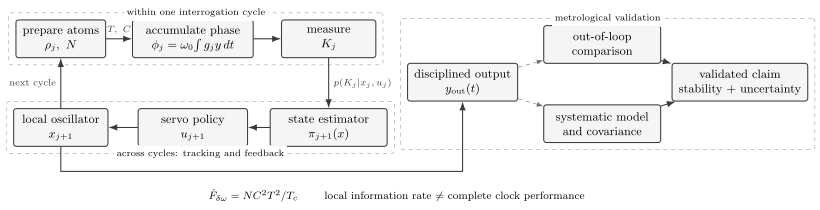
Three inference layers coexist. Within a cycle, atoms encode a relative phase and produce an outcome. Across cycles, a state estimator tracks the noisy local oscillator and a servo chooses the next correction. Outside the loop, an independent comparison and a systematic model determine which stability and uncertainty claims are justified.

An in-loop error signal can be small because feedback suppresses it. That does not independently demonstrate that the output is correct. A trustworthy clock requires a second measurement path, a comparison with another reference, or a validated model showing how the in-loop record predicts out-of-loop behavior.

The Per-Cycle Phase Channel

Let the local oscillator have instantaneous fractional frequency offset

$$y_{\mathrm{LO}}(t) = \frac{\omega_{\mathrm{LO}}(t)-\omega_0}{\omega_0}.$$

During cycle $j$, the interrogation sensitivity function $g_j(t)$ weights oscillator fluctuations. A useful relative-phase model is

$$\phi_j = \omega_0 \int_{t_j}^{t_j+T_c} g_j(t)y_{\mathrm{LO}}(t)\,dt + \phi_{\mathrm{sys},j} + \phi_{\mathrm{ctrl},j}.$$

Here $T_c$ is the full cycle time, $\phi_{\mathrm{sys},j}$ collects atomic and apparatus shifts, and $\phi_{\mathrm{ctrl},j}$ is the known analysis or servo phase. For ideal Ramsey free evolution of duration $T$, $g_j(t)=1$ during the dark interval and zero elsewhere, so a constant detuning gives

$$\phi_j=\delta\omega_jT+\phi_{\mathrm{sys},j} +\phi_{\mathrm{ctrl},j}.$$

For $N$ independent two-level atoms and state-resolved population detection, the excited count $K_j$ is approximately binomial:

$$K_j\sim\operatorname{Binomial} \!\left(N,p_e(\phi_j)\right),$$

with an effective Ramsey fringe

$$p_e(\phi_j) = \frac{1+C\sin\phi_j}{2}$$

when the analysis phase places the clock at quadrature. Contrast $C$ can include dephasing, pulse errors, inhomogeneity, and unresolved oscillator phase noise. Detection errors require a response model rather than an unexplained replacement $C<1$.

The atomic outcome is not a direct observation of instantaneous frequency. It is a noisy, periodic observation of an integrated phase. This distinction is central to clock design.

Phase and Frequency Information

For one atom with the quadrature likelihood above, the phase FI is $C^2$ at $\phi=0$. For $N$ independent atoms,

$$F_\phi^{\mathrm{CSS}} = NC^2,$$

where CSS denotes a coherent spin state. Since $\phi=\delta\omega T$, information transforms as

$$F_{\delta\omega}^{\mathrm{CSS}} = NC^2T^2.$$

If independent cycles of duration $T_c$ can be combined and the oscillator model does not introduce an additional limit, the information rate is

$$\dot F_{\delta\omega} = \frac{NC^2T^2}{T_c}.$$

Writing the duty factor as $D=T/T_c$ gives

$$\dot F_{\delta\omega} = NC^2TD.$$

This formula makes four levers visible: atom number, contrast, interrogation time, and duty factor. It also prevents preparation and readout time from disappearing when two protocols are compared.

For averaging time $\tau\gg T_c$, the corresponding atom-projection-noise benchmark for fractional frequency is

$$\sigma_y^{\mathrm{QPN}}(\tau) \simeq \frac{1}{\omega_0CT\sqrt N} \sqrt{\frac{T_c}{\tau}}.$$

The numerical prefactor depends on the modulation, line shape, estimator, and definition of one error sample. This is an independent-atom benchmark under a local, correctly locked model. It is not automatically the instability of a running clock.

The high carrier frequency of an optical transition improves fractional frequency sensitivity through the factor $1/\omega_0$. It does not by itself remove laser noise, systematic shifts, dead time, or transfer uncertainty.

The Clock as a State-Space Model

Successive clock cycles are generally not independent. Oscillator frequency noise has memory, the servo feeds previous outcomes into future controls, and slow systematic variables drift. A state-space model makes these dependencies explicit. Let $x_j$ contain the latent oscillator offset, drift, and selected nuisance parameters. Then

$$\begin{aligned} x_{j+1} &= f(x_j,u_j)+w_j, \\ K_j &\sim p(K_j|x_j,u_j), \end{aligned}$$

where $u_j$ is the applied control and $w_j$ is process noise. A Bayesian filter updates

$$\pi_{j+1}(x) \propto p(K_j|x,u_j) \int p(x|x',u_j)\pi_j(x')\,dx'.$$

The controller chooses $u_{j+1}$ from this posterior or a sufficient statistic such as its mean and covariance. In a narrow, approximately linear and Gaussian regime this becomes a Kalman filter; broad periodic posteriors may require a circular, grid-based, or particle representation.

A scalar example shows why measurement precision and oscillator quality must be optimized together. Suppose the latent cycle-to-cycle frequency follows a random walk,

$$x_{j+1}=x_j+w_j, \qquad \operatorname{Var}(w_j)=q,$$

and a locally linear atomic readout is

$$r_j=x_j+v_j, \qquad \operatorname{Var}(v_j)=R.$$

If $P$ is the steady-state posterior variance, prediction gives $P+q$ and measurement update gives

$$P = \frac{R(P+q)}{P+q+R}.$$

The nonnegative solution is

$$P = \frac{ \sqrt{q^2+4qR}-q }{2}.$$

Reducing atomic measurement noise $R$ helps, but the gain depends on process noise $q$. When $q$ is large, oscillator unpredictability replenishes uncertainty between observations. When $q$ is very small, the filter can average many weak measurements coherently. A clock-level optimization must include both.

Local Oscillator Noise Is Part of the Task

The local oscillator is not merely a technical imperfection external to quantum metrology. Its phase is precisely what the atoms are asked to estimate and stabilize. Oscillator noise can

• broaden the phase prior before each measurement;
• reduce observed contrast when untracked;
• drive the state outside the discriminator’s local range;
• correlate outcomes from different cycles;
• enter through pulse phases and optical-path delivery;
• be aliased by dead time; and
• set the benefit obtainable from lower atomic readout noise.

If an untracked Gaussian phase has variance $\sigma_{\mathrm{LO}}^2(T)$, its average coherence factor is

$$C_{\mathrm{LO}}(T) = \exp\!\left[ -\frac{\sigma_{\mathrm{LO}}^2(T)}{2} \right].$$

Substituting this factor into a fringe model captures contrast loss but not every consequence of colored oscillator noise. The same noise also determines the phase prior, cycle-to-cycle correlations, and slip probability. A full clock model therefore uses a phase-noise or fractional-frequency-noise spectrum and the actual sensitivity function. Noise Spectra develops spectral conventions; the AMO Atomic Clocks page owns the clock-specific Dick-effect sum.

Dead time and aliasing

Preparation and detection create intervals during which the atoms do not observe the oscillator. Periodic sampling mixes local-oscillator noise near harmonics of $1/T_c$ into the clock record: the Dick effect. Increasing $N$ or squeezing the atomic readout does not suppress that aliased oscillator noise. Indeed, reducing projection noise can reveal a Dick-noise floor that was previously hidden.

Important mitigation strategies have different resource costs:

• faster preparation and readout raise duty factor;
• interleaved ensembles can provide nearly continuous sensitivity;
• a quieter oscillator reduces phase diffusion but may require a larger cryogenic, optical, or vibration-isolated subsystem;
• synchronous comparison rejects shared oscillator noise but changes the claim from independent stability to differential stability;
• nondestructive or weak measurements can track phase while adding measurement backaction and control complexity.

Zero dead time is therefore an architecture claim, not a free change to $T_c=T$. The extra ensemble, controls, optical paths, and failure modes belong in the resource and uncertainty ledgers.

Phase Wraps and Clock Reliability

A two-outcome Ramsey fringe is periodic. Near a chosen operating point the error signal is approximately linear, but outside its capture interval the same measurement can indicate the wrong branch. If a clock accepts phases only within $|\phi|<\phi_{\mathrm{cap}}$ and the predicted phase is Gaussian with standard deviation $\sigma_\phi$, the approximate slip probability per cycle is

$$P_{\mathrm{slip}} \simeq \operatorname{erfc}\!\left( \frac{\phi_{\mathrm{cap}}}{\sqrt2\sigma_\phi} \right).$$

Even a small per-cycle probability can dominate a long data set. If there are $M$ nearly independent opportunities to slip, then

$$P(\text{at least one slip}) = 1-(1-P_{\mathrm{slip}})^M \simeq MP_{\mathrm{slip}}$$

when $MP_{\mathrm{slip}}\ll1$.

Longer interrogation increases local frequency information as $T^2$ but also widens the oscillator phase distribution and narrows the unambiguous frequency range. Multi-ensemble protocols can use short or dual-quadrature interrogations to identify the branch for a longer interrogation. Adaptive protocols can carry a full phase posterior and choose $T$ or analysis phase from its width. Every auxiliary ensemble and short interrogation counts toward the global resource comparison.

A clock that occasionally makes undetected fringe hops may have an impressive conditional Allan deviation after bad runs are removed. Reliability claims must report the detection rule, removed intervals, false-alarm rate, recovery time, and effect on availability.

Choosing the Interrogation Time

If independent atomic coherence decays as

$$C(T)=e^{-\Gamma T},$$

then the ideal CSS information rate is

$$\dot F_{\delta\omega}(T) = \frac{NT^2e^{-2\Gamma T}}{T+t_d},$$

where $t_d=T_c-T$ is fixed dead time. The optimal $T$ solves

$$\frac{2}{T} - 2\Gamma - \frac{1}{T+t_d} =0.$$

With zero dead time, $T_*=1/(2\Gamma)$. Positive dead time makes longer interrogations relatively more valuable because each cycle carries fixed overhead. Oscillator phase wraps or non-Markovian noise can impose a shorter optimum than this contrast-only model predicts.

This optimization illustrates a recurring rule: maximize information or task utility per wall-clock resource, not information per successful interrogation in isolation.

Entangled Probes in a Clock

For a collective spin $J_z=\frac12\sum_{n=1}^N\sigma_z^{(n)}$ and frequency encoding

$$U_{\delta\omega}(T) = e^{-i\delta\omega TJ_z},$$

the pure-state frequency QFI is

$$F_{\delta\omega} = 4T^2\operatorname{Var}(J_z).$$

A CSS has $\operatorname{Var}(J_z)=N/4$ and $F=N T^2$. An ideal GHZ state has $\operatorname{Var}(J_z)=N^2/4$ and

$$F_{\delta\omega}^{\mathrm{GHZ}} = N^2T^2.$$

The ideal local gain comes with three clock-specific liabilities:

1. the GHZ fringe repeats $N$ times faster, reducing capture range;
2. independent decoherence generally destroys its coherence faster;
3. preparation, verification, and readout consume time and may fail.

Under independent Markovian dephasing at rate $\Gamma$, a simple product-state model has contrast $e^{-\Gamma T}$, while GHZ coherence decays as $e^{-N\Gamma T}$. With no dead time, their information rates are

$$\begin{aligned} \dot F_{\mathrm{CSS}} &= NT e^{-2\Gamma T}, \\ \dot F_{\mathrm{GHZ}} &= N^2T e^{-2N\Gamma T}. \end{aligned}$$

Optimizing gives

$$T_{\mathrm{CSS}}^* = \frac{1}{2\Gamma}, \qquad T_{\mathrm{GHZ}}^* = \frac{1}{2N\Gamma},$$

and both reach

$$\dot F^* = \frac{N}{2e\Gamma}.$$

This model does not say entanglement is never useful. It says that ideal $N^2$ single-shot QFI does not by itself establish an asymptotic clock gain under independent Markovian dephasing. Finite-$N$ states, correlated noise, error correction, collective measurements, or different resource constraints can change the optimum, but each requires its own channel model.

Spin squeezing

A spin-squeezed state is often more practical than a GHZ state. Its Wineland parameter

$$\xi_R^2 = \frac{N(\Delta J_\perp)^2}{|\langle\mathbf J\rangle|^2}$$

already compares noise with signal response. In a locally linear Ramsey measurement, an idealized phase variance is

$$(\Delta\phi)^2 \simeq \frac{\xi_R^2}{N},$$

or an effective information $F_\phi\simeq N/\xi_R^2$. Spin Squeezing owns the covariance geometry, entanglement witnesses, preparation methods, readout, and gain calibration.

A clock-level advantage additionally requires that squeezing improve the closed-loop output after including

• preparation time and duty factor;
• contrast and atom loss;
• detection noise and finite dynamic range;
• local-oscillator phase diffusion;
• anti-squeezing coupled through phase error;
• estimator and servo behavior;
• success probability and discarded cycles; and
• the matched unsqueezed clock protocol.

Reducing atomic phase noise below the CSS level is an important result. It is not identical to demonstrating lower Allan deviation for an independently operating clock.

The Clock Resource Ledger

A reproducible comparison should state at least:

Resource	Why it matters
Atom number $N$ and accepted atom distribution	Sets projection noise, interactions, and density-related behavior
Interrogation time $T$ and cycle time $T_c$	Set phase gain, duty factor, bandwidth, and aliasing
Total averaging time $\tau$ and uptime	Determine statistical reach and availability
Contrast and detection response	Determine the implemented likelihood and FI
Oscillator noise spectrum and coherence	Set prior width, correlations, and phase-slip risk
Preparation and entangling time	Can erase a per-shot quantum gain in information per time
Failed preparations and rejected cycles	Must enter throughput and selection accounting
Control and estimator policy	Determine lock range, bias, and steady-state behavior
Auxiliary ensembles and references	Enable unwrapping, zero dead time, or common-mode rejection
Systematic-calibration data	Connect the locked output to the intended unperturbed transition

The appropriate denominator depends on the claim. For a transportable clock it may include size, power, thermal load, or availability. For a lattice clock it may include atom loading, collision constraints, and laser infrastructure. For a fundamental-physics comparison it may include coherent-link uptime and the uncertainty of sensitivity coefficients. No single scalar resource captures all these tasks.

Synchronous and Independent Comparisons

Two clocks interrogated synchronously by a shared local oscillator can reject common oscillator phase. A simplified differential phase is

$$d_j = (\omega_A-\omega_B)T + n_{A,j}-n_{B,j} + \phi_{\mathrm{link},j},$$

where the common oscillator term has canceled. This can reveal atomic projection noise or a frequency ratio beneath the free-running oscillator noise. It is a powerful comparison architecture, but it does not directly show how either clock would perform with an independent oscillator.

For two fractional-frequency estimates with covariance, the differential variance is

$$\operatorname{Var}(y_A-y_B) = \operatorname{Var}(y_A) + \operatorname{Var}(y_B) - 2\operatorname{Cov}(y_A,y_B).$$

Ignoring the covariance can either exaggerate or hide noise. Shared lasers, environmental monitors, atom preparation, transfer links, and data processing all create correlations. Conversely, an independent comparison includes both clocks and the link; attributing the result to one clock requires an additional model or a third reference.

The same distinction applies to entanglement-enhanced comparisons. A differential gain with a common oscillator establishes a valuable network or ratio result under that architecture. A claim about stand-alone timekeeping must include the oscillator and control resources needed at each node.

Stability, Accuracy, and Estimator Risk

Define fractional frequency deviation

$$y(t)=\frac{\nu(t)-\nu_0}{\nu_0}.$$

For adjacent averages $\bar y_k(\tau)$, Allan variance is

$$\sigma_y^2(\tau) = \frac12 \mathbb E\!\left[ (\bar y_{k+1}-\bar y_k)^2 \right].$$

It is a stability statistic for a specified record and averaging time. It is not automatically a frequentist confidence interval for the mean, a Bayesian posterior width, or a systematic uncertainty. Drift, flicker floors, gaps, servo transients, and selection can all invalidate a casual $1/\sqrt\tau$ extrapolation.

Systematic accuracy is a separate estimation problem. A schematic clock measurement equation is

$$y_{\mathrm{corr}} = y_{\mathrm{meas}} - \sum_r \beta_r x_r,$$

where $x_r$ are environmental or operating variables and $\beta_r$ are sensitivities. Uncertainty in both, together with covariance, propagates to the corrected result. Quantum Fisher information for the Ramsey phase does not bound an unmodeled bias. Detailed shift evaluation belongs to the AMO clock pages.

A mature result therefore keeps at least four objects separate:

• single-cycle phase resolution;
• locked-clock instability versus averaging time;
• systematic uncertainty of the realized frequency;
• task loss, such as time error, ratio uncertainty, availability, or anomaly-detection probability.

Optimizing one does not guarantee improvement in the others.

A Worked Quantum-Gain Audit

Consider an optical clock with

$$\nu_0=4.3\times10^{14}\,\mathrm{Hz}, \quad N=10^4, \quad T=0.50\,\mathrm{s},$$

$C=0.80$, and $T_c=1.0\,\mathrm{s}$. The CSS projection-noise benchmark at $\tau=1\,\mathrm{s}$ is

$$\begin{aligned} \sigma_y^{\mathrm{QPN}}(1\,\mathrm{s}) &\simeq \frac{1}{ 2\pi(4.3\times10^{14})(0.80)(0.50)(100) } \\ &\simeq 9.3\times10^{-18}. \end{aligned}$$

Suppose a squeezed protocol has metrological parameter $\xi_R^2=10^{-5/10}\simeq0.316$ but increases cycle time to $1.20\,\mathrm{s}$. If all other clock noise is absent and $\xi_R^2$ already includes the response reduction, the ratio of squeezed to CSS instability is

$$\frac{\sigma_y^{\mathrm{sq}}}{\sigma_y^{\mathrm{CSS}}} = \sqrt{\xi_R^2} \sqrt{\frac{1.20}{1.00}} \simeq 0.616.$$

The idealized clock-level improvement is therefore about $1/0.616\simeq1.62$, not the $10^{5/20}\simeq1.78$ phase-amplitude gain inferred from $5$ dB alone. If Dick noise or oscillator phase slips already exceed the CSS projection-noise term, the total improvement is smaller and may vanish.

What Different Demonstrations Establish

Demonstration	Establishes	Still needed for the next claim
Entanglement witness or $\xi_R^2<1$	Nonclassical collective state and possible local metrological gain	Ramsey response, contrast, and implemented readout
Reduced atomic phase variance	Better single-cycle phase estimate under stated conditions	Preparation time, failures, oscillator noise, and phase range
Higher FI per completed cycle	Better local likelihood per cycle	Information per wall time and global lock reliability
Lower synchronous comparison noise	Better differential performance with common-mode rejection	Independent oscillator performance and covariance audit
Lower locked-clock Allan deviation	Better stability over a stated averaging range	Systematic uncertainty, uptime, and out-of-loop validation
Smaller evaluated uncertainty	Better realization of the stated transition	Traceability, independent agreement, and application utility

An end-to-end quantum clock claim should publish the unsqueezed comparator, atom-number distributions, cycle sequence, preparation success, full outcome record, oscillator spectrum, servo law, phase-slip handling, dead-time model, Allan or likelihood analysis, out-of-loop comparison, and systematic budget. Subtraction of independently estimated oscillator noise can reveal atomic performance, but the result must be labeled as a noise-subtracted atomic or differential metric rather than an unconditional clock output.

Common Mistakes

• Saying that atoms tick continuously in a passive clock.
• Treating repeated cycles as independent when oscillator noise and feedback correlate them.
• Calling the QPN formula the clock’s measured instability without showing that oscillator, detection, and Dick noise are lower.
• Maximizing $T^2$ phase gain while ignoring contrast, cycle time, and phase wraps.
• Quoting squeezing in decibels without using a response-aware metrological parameter.
• Comparing a squeezed cycle with an unsqueezed cycle that has different atom number, duty factor, or acceptance rules.
• Calling a common-oscillator differential comparison an independent clock stability measurement.
• Removing fringe hops or failed preparations without counting their frequency, detection rule, and recovery time.
• Interpreting Allan deviation as systematic accuracy or as a universal uncertainty of the mean.
• Treating a small in-loop residual as independent proof of a correct output.
• Using ideal GHZ QFI without counting the shortened coherence time and $N$-fold phase ambiguity.
• Claiming a redefinition of the SI second from an optical-clock performance result; definitions and realization policy are metrological decisions.

Exercises

1. CSS and GHZ frequency information

For $N$ two-level atoms interrogated for time $T$, calculate the ideal frequency QFI of a CSS and a GHZ state. What additional issue appears in the GHZ likelihood?

Solution

Frequency is encoded by $e^{-i\delta\omega TJ_z}$, so

$$F_{\delta\omega} = 4T^2\operatorname{Var}(J_z).$$

For a CSS, $\operatorname{Var}(J_z)=N/4$, giving

$$F_{\delta\omega}^{\mathrm{CSS}}=NT^2.$$

For a GHZ state, $\operatorname{Var}(J_z)=N^2/4$, giving

$$F_{\delta\omega}^{\mathrm{GHZ}}=N^2T^2.$$

The GHZ signal depends on $N\delta\omega T$, so its unambiguous detuning range is reduced by a factor $N$. The local QFI does not resolve those branches.

2. Projection-noise benchmark

A Ramsey clock has $N=2500$, $C=0.75$, $T=0.20\,\mathrm{s}$, $T_c=0.50\,\mathrm{s}$, and $\nu_0=9.192631770\,\mathrm{GHz}$. Estimate its QPN-limited Allan deviation at $\tau=100\,\mathrm{s}$.

Solution

Use

$$\sigma_y^{\mathrm{QPN}}(\tau) = \frac{1}{2\pi\nu_0CT\sqrt N} \sqrt{\frac{T_c}{\tau}}.$$

Substitution gives

$$\begin{aligned} \sigma_y^{\mathrm{QPN}}(100\,\mathrm{s}) &= \frac{ \sqrt{0.50/100} }{ 2\pi(9.192631770\times10^9)(0.75)(0.20)(50) } \\ &\simeq 1.63\times10^{-13}. \end{aligned}$$

This is a projection-noise benchmark. It omits oscillator noise, Dick aliasing, detection noise, shifts, and servo dynamics.

3. Optimum interrogation with dephasing

Assume zero dead time and $C(T)=e^{-\Gamma T}$. Maximize the CSS frequency information rate and find its maximum.

Solution

With $T_c=T$,

$$\dot F(T)=NTe^{-2\Gamma T}.$$

Differentiating,

$$\frac{d\dot F}{dT} = Ne^{-2\Gamma T}(1-2\Gamma T).$$

Thus

$$T_*=\frac{1}{2\Gamma},$$

and

$$\dot F(T_*) = \frac{N}{2e\Gamma}.$$

The result assumes independent Markovian dephasing and no phase-wrap or oscillator constraint.

4. Fixed overhead shifts the optimum

For $\Gamma=1\,\mathrm{s}^{-1}$ and fixed dead time $t_d=0.20\,\mathrm{s}$, solve the interrogation-time condition

$$\frac2T-2\Gamma-\frac1{T+t_d}=0.$$

Solution

Multiplying by $T(T+t_d)$ gives

$$2(T+t_d)-2\Gamma T(T+t_d)-T=0.$$

With the stated values,

$$2T^2-0.6T-0.4=0.$$

The positive root is

$$T_* = \frac{0.6+\sqrt{0.36+3.2}}{4} \simeq 0.622\,\mathrm{s}.$$

This exceeds the zero-dead-time optimum $0.5\,\mathrm{s}$ because a longer interrogation amortizes the fixed overhead.

5. Steady-state tracking variance

For the scalar random-walk clock model, let process variance be $q=4\times10^{-4}$ and atomic measurement variance be $R=9\times10^{-4}$. Find the steady-state posterior variance $P$ and standard deviation.

Solution

Use

$$P = \frac{\sqrt{q^2+4qR}-q}{2}.$$

Then

$$\begin{aligned} P &= \frac{ \sqrt{(4\times10^{-4})^2 +4(4\times10^{-4})(9\times10^{-4})} -4\times10^{-4} }{2} \\ &\simeq 4.32\times10^{-4}. \end{aligned}$$

Therefore

$$\sqrt P\simeq2.08\times10^{-2}.$$

The posterior variance is neither $q$ nor $R$; it is set by their dynamical balance.

6. Long-run phase-slip risk

A clock has Gaussian predicted phase with $\sigma_\phi=0.25\,\mathrm{rad}$ and capture half-width $\phi_{\mathrm{cap}}=\pi/2$. Estimate the per-cycle slip probability and explain why a long-run report must still monitor slips.

Solution

The Gaussian-tail estimate is

$$P_{\mathrm{slip}} \simeq \operatorname{erfc}\!\left( \frac{\pi/2}{\sqrt2(0.25)} \right) = \operatorname{erfc}(4.44).$$

Numerically this is approximately

$$P_{\mathrm{slip}} \simeq 3.4\times10^{-10}$$

per independent opportunity. Over $10^9$ cycles, the small-probability estimate gives an expected slip count of order $0.34$ and probability $1-e^{-0.34}\simeq0.29$ of at least one slip. Very small per-cycle risks can therefore matter in long operation.

7. A synchronous comparison

Two clocks have individual fractional-frequency variances $9$ and $16$ in arbitrary units and covariance $10$ because they share a local oscillator. Find the variance of their difference. What value would be inferred if the covariance were ignored?

Solution

The differential variance is

$$\operatorname{Var}(y_A-y_B) = 9+16-2(10) = 5.$$

Ignoring covariance would give $25$, five times too large. The shared oscillator can be strongly rejected in the difference. The low differential variance does not imply that either stand-alone output has variance $5$.

8. Audit a squeezed-clock claim

An experiment reports $6\,\mathrm{dB}$ of spin squeezing and a Ramsey phase variance below the CSS level after subtracting independently estimated laser noise. List at least eight additional items needed for an unconditional claim of improved clock stability.

Solution

A clock-level audit should include at least:

1. the response-aware $\xi_R^2$, including contrast and atom-number normalization;
2. preparation time and total cycle time for both protocols;
3. failed preparations, rejected cycles, and recovery time;
4. the local-oscillator spectrum without subtraction;
5. the servo and estimator used in each clock;
6. phase-slip detection, false alarms, and full capture range;
7. Dick-noise and detector-noise budgets;
8. Allan deviation of the actual locked outputs over a stated range;
9. an out-of-loop or independent comparison;
10. matched atom number, interrogation time, and uptime;
11. the systematic-shift and uncertainty ledgers; and
12. raw-data and uncertainty procedures sufficient to reproduce the claim.

The reported result can already establish useful atomic metrological gain. Noise subtraction and conditional analysis must remain visible in the claim.

References

1. N. F. Ramsey, “A molecular beam resonance method with separated oscillating fields,” Physical Review 78, 695–699 (1950), doi:10.1103/PhysRev.78.695.
2. D. W. Allan, “Statistics of atomic frequency standards,” Proceedings of the IEEE 54, 221–230 (1966), doi:10.1109/PROC.1966.4634.
3. W. M. Itano, J. C. Bergquist, J. J. Bollinger, J. M. Gilligan, D. J. Heinzen, F. L. Moore, M. G. Raizen, and D. J. Wineland, “Quantum projection noise: Population fluctuations in two-level systems,” Physical Review A 47, 3554–3570 (1993), doi:10.1103/PhysRevA.47.3554.
4. D. J. Wineland, J. J. Bollinger, W. M. Itano, F. L. Moore, and D. J. Heinzen, “Spin squeezing and reduced quantum noise in spectroscopy,” Physical Review A 46, R6797–R6800 (1992), doi:10.1103/PhysRevA.46.R6797.
5. S. F. Huelga, C. Macchiavello, T. Pellizzari, A. K. Ekert, M. B. Plenio, and J. I. Cirac, “Improvement of frequency standards with quantum entanglement,” Physical Review Letters 79, 3865–3868 (1997), doi:10.1103/PhysRevLett.79.3865.
6. G. Santarelli, C. Audoin, A. Makdissi, P. Laurent, G. J. Dick, and A. Clairon, “Frequency stability degradation of an oscillator slaved to a periodically interrogated atomic resonator,” IEEE Transactions on Ultrasonics, Ferroelectrics, and Frequency Control 45, 887–894 (1998), doi:10.1109/58.710548.
7. G. Santarelli, Ph. Laurent, P. Lemonde, A. Clairon, A. G. Mann, S. Chang, A. N. Luiten, and C. Salomon, “Quantum projection noise in an atomic fountain: A high stability cesium frequency standard,” Physical Review Letters 82, 4619–4622 (1999), doi:10.1103/PhysRevLett.82.4619.
8. M. G. A. Paris, “Quantum estimation for quantum technology,” International Journal of Quantum Information 7, 125–137 (2009), doi:10.1142/S0219749909004839.
9. A. D. Ludlow, M. M. Boyd, J. Ye, E. Peik, and P. O. Schmidt, “Optical atomic clocks,” Reviews of Modern Physics 87, 637–701 (2015), doi:10.1103/RevModPhys.87.637.
10. M. Schioppo et al., “Ultrastable optical clock with two cold-atom ensembles,” Nature Photonics 11, 48–52 (2017), doi:10.1038/nphoton.2016.231.
11. E. Oelker et al., “Demonstration of $4.8\times10^{-17}$ stability at 1 s for two independent optical clocks,” Nature Photonics 13, 714–719 (2019), doi:10.1038/s41566-019-0493-4.
12. E. Pedrozo-Peñafiel et al., “Entanglement on an optical atomic-clock transition,” Nature 588, 414–418 (2020), doi:10.1038/s41586-020-3006-1.
13. M. Schulte, C. Lisdat, P. O. Schmidt, U. Sterr, and K. Hammerer, “Prospects and challenges for squeezing-enhanced optical atomic clocks,” Nature Communications 11, 5955 (2020), doi:10.1038/s41467-020-19403-7.
14. E. M. Kessler, P. Kómár, M. Bishof, L. Jiang, A. S. Sørensen, J. Ye, and M. D. Lukin, “Heisenberg-limited atom clocks based on entangled qubits,” Physical Review Letters 112, 190403 (2014), doi:10.1103/PhysRevLett.112.190403.
15. L. Pezzè, A. Smerzi, M. K. Oberthaler, R. Schmied, and P. Treutlein, “Quantum metrology with nonclassical states of atomic ensembles,” Reviews of Modern Physics 90, 035005 (2018), doi:10.1103/RevModPhys.90.035005.
16. W. J. Eckner et al., “Realizing spin squeezing with Rydberg interactions in an optical clock,” Nature 621, 734–739 (2023), doi:10.1038/s41586-023-06360-6.
17. J. M. Robinson et al., “Direct comparison of two spin-squeezed optical clock ensembles at the $10^{-17}$ level,” Nature Physics 20, 208–213 (2024), doi:10.1038/s41567-023-02310-1.
18. Bureau International des Poids et Mesures, The International System of Units (SI Brochure), 9th ed., version 4.01 (2026), doi:10.59161/AUEZ1291.

Further Connections

• Atomic Clocks owns physical clock architectures, microwave and optical comparisons, the Dick-effect derivation, systematic shifts, the SI second, and complete uncertainty budgets.
• Optical Clocks develops ion and lattice platforms, clock lasers, frequency combs, optical ratios, geodesy, and tests of fundamental physics.
• Frequency Standards develops Allan-family statistics, traceability, time scales, holdover, and frequency-transfer chains.
• Ramsey Interferometry owns the binary likelihood, Fisher information, phase aliases, adaptive interrogation, and information-per-time analysis used in each cycle.
• Spin Squeezing owns collective-spin covariance, Wineland gain, entanglement certification, squeezing preparation, and readout diagnostics.
• Standard Quantum Limit defines the matched independent-atom benchmark and distinguishes constant gains from changed asymptotic scaling.
• Heisenberg Scaling treats GHZ probes, parallel and sequential queries, global phase risk, nonlinear encodings, and noisy bounds.
• Distributed Quantum Sensing treats remote-clock differences as weighted network estimands and audits inter-node entanglement, link success, reference frames, and wall-time information rate.
• Measurement-Based Feedback develops conditional estimation, feedback laws, latency, stability, and in-loop versus out-of-loop evidence.
• Sensing Case Studies compares clock, magnetometer, interferometer, and electrometer claims under shared evidence standards.