Noise and Decoherence in Metrology

Noise in quantum metrology is any uncontrolled or incompletely modeled part of a sensing experiment that changes the distribution of recorded data. It may enter during state preparation, parameter encoding, control, storage, transport, or readout. Decoherence is narrower: it is the loss of off-diagonal coherence in a specified reduced description after degrees of freedom or records are ignored. Dephasing, energy relaxation, particle loss, detector errors, calibration drift, and common-mode fluctuations can all limit a sensor, but they are not interchangeable mechanisms.

The metrological question is also more precise than “how much coherence survives?” A useful sensor must keep states corresponding to nearby parameter values distinguishable, deliver that distinguishability through an available measurement, and do so at a favorable rate after every probe, second, calibration, and failed trial is counted. A channel may destroy one kind of coherence while preserving the signal, or preserve a beautiful state while erasing the derivative that carried the signal.

This page is the canonical home for the synthesis between open-system noise and metrological performance. It develops noisy-channel estimation, information per unit time, dephasing and photon-loss limits, independent and correlated noise, short-time departures from Markovian scaling, control, environment monitoring, and error-corrected sensing. Quantum Channels and Noise owns the channel formalism and individual noise models. Noise Spectra owns spectral conventions, while Classical and Quantum Fisher Information owns the information geometry used here.

The Noisy Estimation Contract

Write one controlled use of a sensor as a parameterized channel

$$\rho_{\theta,\boldsymbol\lambda}^{(u)} = \mathcal E_{\theta,\boldsymbol\lambda}^{(u)}(\rho_0),$$

followed by a POVM $\{M_x^{(u)}\}$. The controls $u$ include preparation, interrogation time, pulse sequence, ancillary systems, and measurement setting. The nuisance vector $\boldsymbol\lambda$ may include dephasing rates, loss, contrast, detuning drift, temperature, and calibration coefficients. The actual likelihood is

$$p(x\mid\theta,\boldsymbol\lambda,u) = \operatorname{Tr} \left[ M_x^{(u)} \mathcal E_{\theta,\boldsymbol\lambda}^{(u)}(\rho_0) \right].$$

This formula prevents several common category errors. Noise is not an additive scalar attached after an ideal sensitivity calculation. It changes the state family, and therefore changes its derivatives, optimal measurement, likelihood support, nuisance correlations, and sometimes the meaning of a resource.

Four questions before calculating a limit

1. What is estimated? A phase, frequency, field, force, loss, temperature, correlation length, or waveform can couple through different parts of the same dynamics.
2. Which channel family is assumed? State-independent dephasing, optical attenuation, a Lindblad semigroup, quasistatic drift, and a correlated bath imply different bounds.
3. Which operations are allowed? Ancillas, feedback, intermediate control, environment monitoring, adaptive measurements, and recovery operations can change the attainable information.
4. Which resource is fixed? Probe number, incident energy, channel uses, sample exposure, elapsed time, spatial aperture, and successful records are not generally equivalent.

Without these declarations, “decoherence restores the SQL” is at most a heuristic. It is a theorem only for specified channel classes, control sets, and resource limits.

Information Must Be Counted at the Output

For one completed cycle, an implemented measurement has classical Fisher information $F_C$, bounded by the quantum Fisher information $F_Q$ of the output state:

$$F_C(\theta;u) \leq F_Q\!\left[ \mathcal E_{\theta,\boldsymbol\lambda}^{(u)}(\rho_0) \right].$$

If $\nu$ cycles are independent and identically configured, a locally unbiased estimator obeys

$$\operatorname{Var}(\widehat\theta) \geq \frac{1}{\nu F_C} \geq \frac{1}{\nu F_Q}.$$

The second inequality is a device-independent ceiling for the declared output state, not a promise that the available readout attains it. Noise can rotate the optimal measurement with the unknown parameter, make nuisance parameters nearly degenerate with the signal, or leave information in an inaccessible environment.

Data processing, with an important qualification

If a parameter-independent channel $\Lambda$ acts after encoding, QFI is contractive:

$$F_Q[\Lambda(\rho_\theta)] \leq F_Q[\rho_\theta].$$

Discarding a subsystem, adding parameter-independent detector noise, or coarse-graining a record cannot increase the available information. But the qualification matters: when $\Lambda_\theta$ itself depends on the unknown parameter, it can encode information. Thermometry, loss estimation, noise spectroscopy, and estimation of a decay rate use the “noise” as the signal. Contractivity does not compare different parameter-dependent channel families.

Information rate and dead time

Suppose an interrogation lasts $t$, while preparation, reset, readout, and feedback require dead time $t_{\rm d}$. The cycle time is

$$t_{\rm c}=t+t_{\rm d},$$

so a long run of duration $T_{\rm tot}$ contains approximately $\nu=T_{\rm tot}/t_{\rm c}$ cycles. The relevant local objective is then

$$\dot F_C(t) = \frac{F_C(t)}{t+t_{\rm d}}, \qquad \operatorname{Var}(\widehat\theta) \gtrsim \frac{1}{T_{\rm tot}\dot F_C(t)}.$$

Longer interrogation usually increases signal phase but decreases contrast and the number of repetitions. Maximizing per-shot QFI can therefore select a different operating point from maximizing precision per unit wall-clock time.

A Taxonomy That Changes the Answer

Distinction	First diagnostic	Metrological consequence
dephasing vs dissipation	are basis populations preserved?	phase contrast and energy response degrade differently
erasure vs unflagged loss	is the missing probe identified?	a flagged event can enter the likelihood rather than disappear
independent vs correlated noise	how does covariance scale across probes?	information may remain extensive, saturate, or occupy a protected differential mode
semigroup vs time-inhomogeneous dynamics	does $\mathcal E_{t+s}=\mathcal E_t\mathcal E_s$ hold?	short-time behavior can change asymptotic frequency scaling
unmonitored vs monitored environment	are jump, leakage, or bath records observed?	discarded records can contain recoverable information
known vs unknown noise parameters	are rates and contrasts calibrated?	nuisance correlations reduce effective signal information
signal-parallel vs signal-transverse noise	does control suppress both by the same symmetry?	decoupling or correction may preserve the signal, or erase it

For the dynamical distinctions behind the first row, see Dephasing vs Dissipation. For the precise hierarchy of non-Markovian definitions, see What Non-Markovian Means.

Exact Qubit Dephasing Example

Consider a Ramsey qubit initialized in $|+\rangle$, accumulating an unknown angular frequency $\omega$ for time $t$. Let a real coherence envelope $0\leq\eta(t)\leq1$ describe parameter-independent dephasing. Immediately before the final analysis pulse,

$$\rho_\omega(t) = \frac12 \begin{pmatrix} 1 & \eta(t)e^{-i\omega t} \\ \eta(t)e^{i\omega t} & 1 \end{pmatrix}.$$

The QFI for phase $\phi=\omega t$ is $\eta(t)^2$, and the frequency QFI is

$$F_Q^{(1)}(\omega,t) = t^2\eta(t)^2.$$

A quadrature Ramsey measurement attains this local value when its analysis phase is correctly set. For $N$ independent probes in the same cycle,

$$F_{Q,\mathrm{prod}}^{(N)} = N t^2\eta(t)^2.$$

Thus dephasing reduces the information by the square of the surviving coherence in this model. That compact result is not universal: amplitude damping changes populations as well as coherence, and parameter-dependent noise adds derivative terms of its own. The Dephasing Channel page owns the channel and Kraus representations.

Markovian dephasing and the optimal time

For exponential coherence

$$\eta(t)=e^{-\gamma t},$$

and negligible dead time, the product-state information rate is

$$\dot F_{Q,\mathrm{prod}} = N t e^{-2\gamma t}.$$

Its optimum occurs at

$$t_\star^{\mathrm{prod}} = \frac{1}{2\gamma}, \qquad \dot F_{Q,\mathrm{prod}}^{\max} = \frac{N}{2e\gamma}.$$

Now prepare the $N$-qubit GHZ state. The signal phase is amplified to $N\omega t$, but independent dephasing multiplies its one fragile coherence by $\eta(t)^N=e^{-N\gamma t}$. Its per-cycle QFI and rate are

$$F_{Q,\mathrm{GHZ}}^{(N)} = N^2t^2e^{-2N\gamma t}, \qquad \dot F_{Q,\mathrm{GHZ}} = N^2t e^{-2N\gamma t}.$$

The optimum moves to

$$t_\star^{\mathrm{GHZ}} = \frac{1}{2N\gamma}, \qquad \dot F_{Q,\mathrm{GHZ}}^{\max} = \frac{N}{2e\gamma}.$$

The $N$-fold faster phase accumulation is exactly canceled by an $N$-fold shorter useful interrogation. In this idealized model the optimized GHZ and product strategies have the same information rate. State-preparation time, collective readout error, and nonzero dead time generally make the maximally entangled strategy less favorable, while partially entangled or squeezed states can still improve finite-resource constants in broader models.

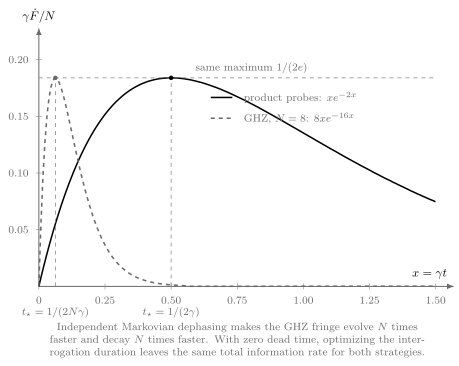
With coherence $e^{-\gamma t}$ and zero dead time, product probes have $\gamma\dot F_Q/N=x e^{-2x}$, while an $N=8$ GHZ probe has $\gamma\dot F_Q/N=8x e^{-16x}$. The optimal times differ by eight, but both curves reach $1/(2e)$. The result compares frequency information per total time, not phase information in a single shot.

Dead time changes the optimization

For exponential decay with coefficient $a$ in the exponent, maximizing

$$\frac{t^2e^{-2at}}{t+t_{\rm d}}$$

gives the positive stationary point

$$t_\star = \frac{ 1-2at_{\rm d} + \sqrt{1+12at_{\rm d}+4a^2t_{\rm d}^2} }{4a}.$$

Use $a=\gamma$ for product probes and $a=N\gamma$ for GHZ probes, together with their different prefactors. A short GHZ interrogation pays the fixed overhead many more times. In clock language, dead time can also alias local oscillator noise into the measurement band; that system effect is not captured by the simple independent-cycle formula.

Readout contrast is another channel

If a symmetric binary readout has net contrast $A$ and is operated at quadrature, its local Fisher information becomes

$$F_C(\omega,t) = A^2 t^2\eta(t)^2.$$

The factors $A$ and $\eta$ may look identical in one fringe, but they arise at different stages and respond differently to controls. A calibration that treats $A$ as known can overstate precision if contrast drift is correlated with frequency. The multiparameter Fisher matrix, not a scalar contrast correction, is then required.

Photon Loss and Fragile Optical States

Loss couples the sensed optical mode to inaccessible modes. It reduces detected energy, leaks which-path information, and turns pure inputs into mixed states. It must be placed at a declared reference plane: source loss, propagation loss, sample absorption, collection loss, and detector inefficiency are physically different even when they share a transmissivity.

For independent photon loss of fixed transmissivity $0<\tau<1$, a standard asymptotic bound for single-parameter optical phase estimation with mean incident photon number $\overline N$ is

$$F_Q \leq \frac{\tau}{1-\tau}\,\overline N, \qquad \Delta\phi \geq \sqrt{ \frac{1-\tau}{\tau\overline N} }.$$

The precise prefactor depends on the interferometer and loss convention, but the scaling statement is robust for the stated independent-loss model: fixed nonzero loss makes the ultimate QFI grow at most linearly with energy. Entanglement and squeezing may still improve the constant, sometimes substantially, but do not restore asymptotic $\overline N^2$ QFI.

The bound becomes loose as $\tau\to1$ and should not be used as a finite-$N$ interpolation formula. It also does not apply unchanged to heralded erasure, correlated loss, monitored environments, nonlinear sample interactions, or a different resource definition.

Why NOON coherence is fragile

In a simple model where every photon must survive for an $N$-photon NOON coherence to remain useful, the surviving coherent branch has weight $\tau^N$. Its phase QFI behaves as

$$F_{Q,\mathrm{NOON}} \sim N^2\tau^N.$$

The $N^2$ ideal sensitivity is eventually overwhelmed by exponential loss. Optimal lossy probes distribute number more gently than a NOON state, and coherent light mixed with squeezed vacuum can approach the relevant large-energy bound in important interferometric regimes. The lesson is not that nonclassical light is useless; it is that the most fragile noiseless optimum is rarely the noisy optimum. See Mach–Zehnder Interferometry for optical probe and measurement details.

Incident, interacting, and detected resources

Three photon numbers should not be silently identified:

$$\overline N_{\rm in}, \qquad \overline N_{\rm sample}, \qquad \overline N_{\rm det}.$$

A photosensitive sample may make $\overline N_{\rm sample}$ the scarce resource, while a remote-sensing link may be limited by transmitted energy and aperture. Detector loss can sometimes be improved without increasing sample exposure. Every quantum and classical comparator must use the same resource boundary.

General Bounds from Channel Geometry

For independent uses of a parameterized channel, bounds can be formulated without optimizing over an exponentially large input state. Let $\{K_j(\theta)\}$ be Kraus operators and dots denote $\theta$ derivatives. Define, for a chosen Kraus representation,

$$\alpha = \sum_j \dot K_j^\dagger\dot K_j, \qquad \beta = i\sum_j \dot K_j^\dagger K_j.$$

Kraus representations are not unique. A parameter-dependent unitary rotation on the environment changes $\alpha$ and $\beta$ without changing the channel. Optimizing over this freedom gives a channel-extension bound of the form

$$F_Q^{(N)} \leq 4\min_h \left[ N\lVert\alpha_h\rVert + N(N-1)\lVert\beta_h\rVert^2 \right].$$

Here $h$ generates the Kraus-space rotation and $\lVert\cdot\rVert$ is the operator norm. If a representation can be chosen with $\beta_h=0$ and bounded $\alpha_h$, the quadratic term vanishes:

$$F_Q^{(N)} \leq 4N\min_{h:\,\beta_h=0} \lVert\alpha_h\rVert.$$

That establishes at-most-linear asymptotic QFI for the specified independent channel, even allowing entangled probes and passive ancillas. It does not say that every measurement attains the bound, and it does not automatically cover correlated channels, adaptive memory effects, or a control model outside the derivation.

These bounds explain why weak local dephasing, depolarization, relaxation, or loss often changes the large-$N$ result discontinuously: ideal quadratic QFI can persist over a finite preasymptotic region, yet the true asymptote is linear. A handful of small-$N$ data points cannot distinguish a long crossover from a new scaling law.

Short-Time Dynamics and the Zeno Scaling

Exponential decay at arbitrarily short times is an idealization. Many microscopic models begin quadratically. Suppose independent dephasing has

$$\eta(t) = 1-c t^\beta+o(t^\beta), \qquad \beta>1.$$

For an $N$-qubit GHZ state at short times,

$$\eta(t)^{2N} \simeq e^{-2Nc t^\beta},$$

and, neglecting dead time, its information rate scales as

$$\dot F_{Q,\mathrm{GHZ}} \simeq N^2t e^{-2Nc t^\beta}.$$

Optimization gives

$$t_\star \propto N^{-1/\beta}, \qquad \dot F_Q^{\max} \propto N^{2-1/\beta}.$$

At fixed total time the variance can therefore scale as $N^{-(2-1/\beta)}$. For quadratic short-time decay, $\beta=2$, this is the Zeno scaling

$$\operatorname{Var}(\widehat\omega) \propto N^{-3/2}, \qquad \Delta\omega \propto N^{-3/4}.$$

This improvement is neither the noiseless Heisenberg law nor a generic reward for “non-Markovianity.” The decisive assumption is the short-time departure from a semigroup, together with access to interrogation times that shrink into that regime. Finite control bandwidth, dead time, spatial correlations, and a later exponential regime can remove the asymptotic window. Information backflow is one possible feature of memory, but it is not the criterion behind the bound above.

Correlated Noise Can Saturate or Protect

Correlations change which collective mode contains signal and which contains noise. A classical Gaussian example already shows the geometry. Let one simultaneous sensor record be

$$\mathbf y = \theta\mathbf s+\boldsymbol\epsilon, \qquad \boldsymbol\epsilon \sim \mathcal N(\mathbf0,\Sigma).$$

Its Fisher information is

$$F_C = \mathbf s^{\mathsf T} \Sigma^{-1} \mathbf s.$$

For a common signal $\mathbf s=\mathbf1$ and covariance

$$\Sigma = \sigma_{\rm i}^2 I + \sigma_{\rm c}^2\mathbf1\mathbf1^{\mathsf T},$$

the result is

$$F_C = \frac{N}{\sigma_{\rm i}^2+N\sigma_{\rm c}^2}.$$

Independent noise alone gives information proportional to $N$. Any fixed common-mode component makes the information saturate at $1/\sigma_{\rm c}^2$ as $N\to\infty$. Treating the records as independent would report fictitious precision.

Conversely, a differential signal vector satisfying $\mathbf1^{\mathsf T}\mathbf s=0$ lies outside the common-noise mode. A differential estimator or decoherence-free subspace can reject that noise. But it also rejects any signal with the same common-mode symmetry. Protection is possible when signal and noise occupy distinguishable operator or spatial subspaces, not merely because noise is correlated. Distributed Quantum Sensing develops this geometry for sensor networks and entangled probes.

Noise Parameters as Nuisance Parameters

Suppose the signal $\theta$ is estimated jointly with unknown contrast, dephasing, or drift parameters $\boldsymbol\lambda$. Partition the Fisher matrix as

$$F = \begin{pmatrix} F_{\theta\theta} & F_{\theta\lambda} \\ F_{\lambda\theta} & F_{\lambda\lambda} \end{pmatrix}.$$

After accounting for nuisance uncertainty, the local information available for $\theta$ is the Schur complement

$$F_{\rm eff} = F_{\theta\theta} - F_{\theta\lambda} F_{\lambda\lambda}^{-1} F_{\lambda\theta}.$$

If the signal derivative resembles a contrast or drift derivative, $F_{\rm eff}$ can be much smaller than $F_{\theta\theta}$. Separate calibration data add information to $F_{\lambda\lambda}$, but the associated probes and time belong in an end-to-end resource comparison. A prior can regularize weakly identified nuisance directions, but then the reported bound is Bayesian and prior-dependent.

When decoherence is the signal

For the dephasing qubit above with $\eta=e^{-\gamma t}$ and known phase, the QFI for the decay rate is

$$F_Q(\gamma,t) = \frac{t^2e^{-2\gamma t}} {1-e^{-2\gamma t}}.$$

The channel now encodes $\gamma$ through the Bloch-vector length. Noise spectroscopy and relaxometry exploit this dependence. Calling decoherence purely detrimental would miss the parameter being measured.

Control Is a Signal-and-Noise Filter

A control sequence changes the toggling-frame signal Hamiltonian and the coupling to noise. For classical dephasing noise $\xi(t)$ and a sign-changing control function $y(t)$, the accumulated target phase is

$$\phi_s(T) = \int_0^T dt\,y(t)s(t),$$

while a stationary Gaussian noise model gives a coherence exponent of the form

$$\chi(T) = \frac{1}{2\pi} \int_{-\infty}^{\infty} d\omega\, S_{\xi\xi}(\omega) |Y_T(\omega)|^2.$$

The same modulation $y(t)$ determines both signal response and noise filter. Spin echo suppresses quasistatic detuning, but it also cancels a static signal coupled through the same operator. For AC sensing, pulse timing can make the target add coherently while low-frequency drift cancels. Dynamical Decoupling owns the filter-function derivation and sequence limitations.

Useful control strategies include:

• choosing a clock transition or sweet spot with small nuisance derivative;
• common-mode rejection and differential encoding;
• dynamical decoupling matched to a target waveform;
• adaptive interrogation times that balance range and coherence;
• optimal control that shapes both signal generator and dissipation;
• reservoir engineering or autonomous stabilization;
• monitoring emitted quanta or leakage flags when their records are informative;
• quantum error detection or correction when signal and error actions can be separated.

Every strategy has overhead and bandwidth. Pulse errors, finite duration, ancilla dephasing, recovery latency, and calibration drift belong in the implemented channel, not in a footnote after the ideal result.

Environment Monitoring and Conditional Records

An unconditional master equation averages over possible environment records. If emitted photons, quantum jumps, erasures, or ancilla syndromes are observed, the full record can retain more information than the averaged sensor state. Schematically,

$$\rho_\theta = \sum_r p(r\mid\theta)\rho_{\theta\mid r}.$$

Keeping the classical label $r$ produces a classical-quantum state whose QFI is

$$F_Q^{\rm record} = F_C[p(r\mid\theta)] + \sum_r p(r\mid\theta) F_Q[\rho_{\theta\mid r}].$$

Discarding $r$ cannot increase information. This identity explains why trajectory monitoring, heralded erasure, and syndrome records can outperform an unmonitored reduced-state protocol. It also gives the correct accounting for postselection: a high-information successful branch is weighted by its success probability, and parameter-dependent success itself carries classical information. Quantum Trajectories owns the conditional-state formalism.

Quantum Error-Corrected Sensing

Ordinary quantum error correction protects an unknown logical state. In metrology, recovery must do something subtler: suppress the dominant errors while preserving a nontrivial logical action of the signal Hamiltonian. Correcting the operator that generates the signal can make a perfectly stable but perfectly insensitive sensor.

Consider a finite-dimensional Markovian model

$$\frac{d\rho}{dt} = -i\omega[G,\rho] + \sum_j \left( L_j\rho L_j^\dagger - \frac12\{L_j^\dagger L_j,\rho\} \right).$$

Define the real Lindblad span

$$\mathcal S = \operatorname{span}_{\mathbb R} \left\{ I, L_j^{\rm H}, iL_j^{\rm AH}, (L_j^\dagger L_k)^{\rm H}, i(L_j^\dagger L_k)^{\rm AH} \right\},$$

where $A^{\rm H}=(A+A^\dagger)/2$ and $A^{\rm AH}=(A-A^\dagger)/2$. Under the strong assumptions of noiseless ancillas and arbitrarily fast, accurate control and recovery, Heisenberg scaling in total sensing time is attainable if and only if

$$G\notin\mathcal S.$$

This is the Hamiltonian-not-in-Lindblad-span, or HNLS, condition.

Two one-qubit geometries

If both signal and dephasing act through $Z$,

$$G=Z, \qquad L=\sqrt\gamma\,Z,$$

then $G\in\mathcal S$. Any code that makes $Z$ errors logically invisible also removes the DC $Z$ signal at leading order. Fast ideal QEC cannot restore Heisenberg scaling for that model.

If instead $G=X$ while $L=\sqrt\gamma Z$, then $G\notin\mathcal S$. With a noiseless ancilla, the codewords

$$|0_L\rangle = |+\rangle_S|0\rangle_A, \qquad |1_L\rangle = |-\rangle_S|1\rangle_A$$

send a sensor $Z$ error outside the code space, while $X_S$ acts as a logical $Z_L$ signal. Frequent syndrome extraction can in principle suppress the noise without erasing the signal.

The theorem is not an off-the-shelf hardware guarantee. Real ancillas are noisy; recoveries consume time; controls have finite strength; higher-order errors accumulate; and syndrome measurements can introduce bias. A useful experiment must compare the corrected sensor with the best uncorrected and classical strategies at the same elapsed time, sensing volume, signal exposure, bandwidth, and hardware inventory. Why Quantum Error Correction Is Possible owns the Knill–Laflamme condition and general recovery theory.

Worked Performance Audits

Markovian Ramsey sensor

Take $N=100$ independent qubits, coherence rate $\gamma=10\ \mathrm{s}^{-1}$, total averaging time $T_{\rm tot}=10\ \mathrm s$, and negligible dead time. The optimal product interrogation is

$$t_\star = \frac{1}{2\gamma} = 0.050\ \mathrm s.$$

The total QFI ceiling is

$$F_Q^{\rm tot} = T_{\rm tot} \frac{N}{2e\gamma} \simeq 18.4\ \mathrm{s}^2,$$

so

$$\Delta\omega \geq \frac{1}{\sqrt{F_Q^{\rm tot}}} \simeq 0.233\ \mathrm{rad\,s^{-1}}.$$

An ideal 100-qubit GHZ probe uses $t_\star=1/(2N\gamma)=0.50\ \mathrm{ms}$ and has the same total-QFI ceiling. It requires one hundred times as many preparation and readout cycles. Even a small fixed overhead therefore breaks the formal tie against it.

Lossy optical phase

Let $\tau=0.90$ and $\overline N=10^6$ incident photons. The asymptotic loss bound gives

$$\Delta\phi \geq \sqrt{ \frac{0.10}{0.90\times10^6} } \simeq 3.33\times10^{-4}\ \mathrm{rad}.$$

A coherent-state shot-noise scale based on the detected mean $\tau\overline N$ is approximately $1/\sqrt{\tau\overline N}=1.05\times10^{-3}\ \mathrm{rad}$. Thus this particular ultimate bound allows at most a factor $1/\sqrt{1-\tau}\simeq3.16$ improvement in standard deviation over that benchmark. It does not prove that a realizable source and receiver attain the factor.

Common-mode floor

Set $\sigma_{\rm i}^2=1$ and $\sigma_{\rm c}^2=0.01$ in the correlated Gaussian model. For $N=100$ sensors,

$$F_C = \frac{100}{1+100(0.01)} = 50,$$

rather than the independently modeled value $100$. For $N=1000$, $F_C\simeq90.9$, already near the asymptotic ceiling $100$. Adding sensors cannot average away the shared fluctuation.

What Can Be Claimed

Evidence	Defensible statement	Missing conclusion
longer measured coherence time	the declared protocol preserves a chosen coherence observable longer	improved parameter information or information rate
larger output QFI	an ideal measurement on the modeled output could carry more local information	available readout attains it
larger measured Fisher information per successful shot	accepted records are more informative	per-attempt or per-time advantage
error-corrected logical oscillation	a signal survives repeated recovery in a declared code	net sensitivity advantage after overhead
sub-SQL point	one matched finite-resource benchmark is exceeded	asymptotic scaling advantage
favorable fitted scaling exponent	data support that model over the fitted range	theorem about the large-$N$ limit
noise model predicts a bound	no strategy inside the model can exceed it	the laboratory satisfies the model

A mature report should publish the full likelihood or sufficient statistics, accepted and rejected counts, elapsed times, calibration schedule, noise covariance or spectrum, fitted nuisance parameters, estimator bias and coverage, and the exact classical comparator. Drift should be tested by interleaving strategies and preserving time order, not hidden by pooling all records.

Common Mistakes

Using a coherence time as a sensitivity

$T_2$, visibility, or squeezing is an intermediate diagnostic. Sensitivity also depends on the signal derivative, readout, cycle time, and estimator.

Optimizing a shot instead of a run

The longest interrogation or largest per-shot QFI may lose to a shorter cycle with more repetitions. Optimize $F/(t+t_{\rm d})$ under the actual resource constraint.

Calling every exponential envelope Markovian

An exponential fit over one time window does not prove a semigroup, and a nonexponential fit does not by itself establish information backflow. State the operational model and tested time range.

Treating independent-noise no-go results as universal

Correlated noise, short-time dynamics, monitored environments, controls, and QEC can change the bound. Their assumptions and overhead must be explicit.

Saying non-Markovianity automatically helps

Memory may preserve, return, or further obscure information. For Zeno frequency scaling, the relevant feature is the short-time decay law, not a generic non-Markovian label.

Refocusing the signal

A pulse sequence or code that cancels a nuisance coupled through $G$ also cancels a signal coupled through the same operator unless another temporal, spectral, spatial, or ancillary distinction is available.

Dropping lost and failed trials

Postselection changes conditional precision. Success probability, failure records, and parameter-dependent acceptance must remain in the likelihood and resource ledger.

Quoting an ultimate bound as achieved performance

A QFI or channel-extension bound is a ceiling. It may require an unavailable input, collective measurement, known operating point, ideal ancilla, or asymptotic regime.

Key Results

• Noise belongs inside the parameterized channel and likelihood, not as an after-the-fact sensitivity penalty.
• For a dephased Ramsey qubit with parameter-independent coherence $\eta(t)$, frequency QFI is $t^2\eta(t)^2$.
• Under independent Markovian dephasing and zero dead time, optimized product and GHZ frequency sensing have the same QFI rate $N/(2e\gamma)$.
• Fixed independent photon loss limits asymptotic optical phase QFI to linear growth with incident energy, while still allowing constant-factor quantum gains.
• Independent-channel geometry can rule out quadratic asymptotic QFI even after entangled inputs and passive ancillas are optimized.
• Quadratic short-time decoherence can permit Zeno variance scaling $N^{-3/2}$, but not noiseless Heisenberg scaling.
• Correlated noise can create a common-mode information floor or a protected differential subspace, depending on signal geometry.
• QEC can restore Heisenberg scaling under ideal Markovian control exactly when the signal generator lies outside the Lindblad span.
• Monitoring and postselection help only according to the information in the complete weighted record.

References

1. S. F. Huelga et al., “Improvement of frequency standards with quantum entanglement,” Physical Review Letters 79, 3865–3868 (1997), doi:10.1103/PhysRevLett.79.3865.
2. B. M. Escher, R. L. de Matos Filho, and L. Davidovich, “General framework for estimating the ultimate precision limit in noisy quantum-enhanced metrology,” Nature Physics 7, 406–411 (2011), doi:10.1038/nphys1958.
3. R. Demkowicz-Dobrzański, J. Kołodyński, and M. Guţă, “The elusive Heisenberg limit in quantum-enhanced metrology,” Nature Communications 3, 1063 (2012), doi:10.1038/ncomms2067.
4. J. Kołodyński and R. Demkowicz-Dobrzański, “Efficient tools for quantum metrology with uncorrelated noise,” New Journal of Physics 15, 073043 (2013), doi:10.1088/1367-2630/15/7/073043.
5. R. Demkowicz-Dobrzański and L. Maccone, “Using entanglement against noise in quantum metrology,” Physical Review Letters 113, 250801 (2014), doi:10.1103/PhysRevLett.113.250801.
6. R. Demkowicz-Dobrzański, M. Jarzyna, and J. Kołodyński, “Quantum limits in optical interferometry,” Progress in Optics 60, 345–435 (2015), doi:10.1016/bs.po.2015.02.003.
7. R. Demkowicz-Dobrzański et al., “Quantum phase estimation with lossy interferometers,” Physical Review A 80, 013825 (2009), doi:10.1103/PhysRevA.80.013825.
8. A. W. Chin, S. F. Huelga, and M. B. Plenio, “Quantum metrology in non-Markovian environments,” Physical Review Letters 109, 233601 (2012), doi:10.1103/PhysRevLett.109.233601.
9. K. Macieszczak, “Zeno limit in frequency estimation with non-Markovian environments,” Physical Review A 92, 010102(R) (2015), doi:10.1103/PhysRevA.92.010102.
10. A. Smirne, J. Kołodyński, S. F. Huelga, and R. Demkowicz-Dobrzański, “Ultimate precision limits for noisy frequency estimation,” Physical Review Letters 116, 120801 (2016), doi:10.1103/PhysRevLett.116.120801.
11. P. Sekatski, M. Skotiniotis, J. Kołodyński, and W. Dür, “Quantum metrology with full and fast quantum control,” Quantum 1, 27 (2017), doi:10.22331/q-2017-09-06-27.
12. R. Demkowicz-Dobrzański, J. Czajkowski, and P. Sekatski, “Adaptive quantum metrology under general Markovian noise,” Physical Review X 7, 041009 (2017), doi:10.1103/PhysRevX.7.041009.
13. S. Zhou, M. Zhang, J. Preskill, and L. Jiang, “Achieving the Heisenberg limit in quantum metrology using quantum error correction,” Nature Communications 9, 78 (2018), doi:10.1038/s41467-017-02510-3.
14. E. M. Kessler et al., “Quantum error correction for metrology,” Physical Review Letters 112, 150802 (2014), doi:10.1103/PhysRevLett.112.150802.
15. W. Dür, M. Skotiniotis, F. Fröwis, and B. Kraus, “Improved quantum metrology using quantum error correction,” Physical Review Letters 112, 080801 (2014), doi:10.1103/PhysRevLett.112.080801.
16. T. Unden et al., “Quantum metrology enhanced by repetitive quantum error correction,” Physical Review Letters 116, 230502 (2016), doi:10.1103/PhysRevLett.116.230502.
17. D. Layden, S. Zhou, P. Cappellaro, and L. Jiang, “Ancilla-free quantum error correction codes for quantum metrology,” Physical Review Letters 122, 040502 (2019), doi:10.1103/PhysRevLett.122.040502.
18. A. Altherr and Y. Yang, “Quantum metrology for non-Markovian processes,” Physical Review Letters 127, 060501 (2021), doi:10.1103/PhysRevLett.127.060501.
19. L. Pezzè et al., “Quantum metrology with nonclassical states of atomic ensembles,” Reviews of Modern Physics 90, 035005 (2018), doi:10.1103/RevModPhys.90.035005.
20. G. Tóth and I. Apellaniz, “Quantum metrology from a quantum information science perspective,” Journal of Physics A 47, 424006 (2014), doi:10.1088/1751-8113/47/42/424006.

Further Connections

• Quantum Measurement as Estimation defines the likelihood, estimator, risk, nuisance, and validation contract used here.
• Classical and Quantum Fisher Information derives QFI, measurement attainability, monotonicity, and multiparameter information matrices.
• Cramér–Rao Bounds explains local unbiasedness, finite-sample behavior, nuisance parameters, and Bayesian alternatives.
• Standard Quantum Limit develops the matched independent-probe benchmark and distinguishes constant gain from changed scaling.
• Heisenberg Scaling owns ideal resource scaling, query counting, global ambiguity, and the distinction between finite-range and asymptotic claims.
• Ramsey Interferometry develops the physical likelihood, contrast envelope, filter function, and adaptive timing used by the dephasing example.
• Atomic Clocks adds oscillator noise, servo dynamics, dead time, stability, and systematic uncertainty.
• Quantum Channels and Noise provides Kraus, Choi, Stinespring, and channel-composition tools for the models summarized here.
• Quantum Sensing connects open-system dynamics, platform noise, control, and sensor implementations.
• Claims, Hype, and Evidence Standards gives the broader rules for matching benchmark scope to experimental evidence.

Exercises

Exercise 1: QFI of a dephased Ramsey qubit

For

$$\rho_\phi = \frac12 \left[ I + \eta(\cos\phi\,X+\sin\phi\,Y) \right],$$

with parameter-independent $0\leq\eta<1$, use the qubit Bloch-vector formula

$$F_Q = |\partial_\phi\mathbf r|^2 + \frac{(\mathbf r\cdot\partial_\phi\mathbf r)^2} {1-|\mathbf r|^2}$$

to derive the phase and frequency QFIs.

Solution

The Bloch vector is

$$\mathbf r = \eta(\cos\phi,\sin\phi,0),$$

so

$$\partial_\phi\mathbf r = \eta(-\sin\phi,\cos\phi,0).$$

Therefore $|\partial_\phi\mathbf r|^2=\eta^2$ and $\mathbf r\cdot\partial_\phi\mathbf r=0$. Hence

$$F_Q(\phi)=\eta^2.$$

For $\phi=\omega t$, the chain rule gives

$$F_Q(\omega,t) = \left(\frac{\partial\phi}{\partial\omega}\right)^2 F_Q(\phi) = t^2\eta(t)^2.$$

Exercise 2: Product and GHZ optimization

Under independent Markovian dephasing, verify that product and GHZ probes have the same optimized frequency-information rate when dead time vanishes.

Solution

For product probes,

$$\dot F_{\rm prod} = Nt e^{-2\gamma t}.$$

Differentiation gives

$$\frac{d\dot F_{\rm prod}}{dt} = Ne^{-2\gamma t}(1-2\gamma t),$$

so $t_\star=1/(2\gamma)$ and $\dot F_{\rm prod}^{\max}=N/(2e\gamma)$.

For a GHZ probe,

$$\dot F_{\rm GHZ} = N^2t e^{-2N\gamma t}.$$

Its derivative vanishes at $t_\star=1/(2N\gamma)$, yielding

$$\dot F_{\rm GHZ}^{\max} = N^2 \frac{1}{2N\gamma} e^{-1} = \frac{N}{2e\gamma}.$$

The equal maxima rely on independent exponential dephasing, ideal preparation and readout, continuous choice of $t$, and zero dead time.

Exercise 3: Optimal interrogation with dead time

Maximize

$$f(t)=\frac{t^2e^{-2at}}{t+d}$$

for $a>0$ and $d\geq0$. Check the $d=0$ limit.

Solution

For $t>0$, logarithmic differentiation gives

$$\frac{f'(t)}{f(t)} = \frac{2}{t} -2a -\frac{1}{t+d}.$$

Setting this to zero and clearing denominators gives

$$2at^2+(2ad-1)t-2d=0.$$

The positive root is

$$t_\star = \frac{ 1-2ad+\sqrt{1+12ad+4a^2d^2} }{4a}.$$

At $d=0$, this reduces to $t_\star=1/(2a)$. The other quadratic root is nonpositive and is not an interrogation time.

Exercise 4: Loss bound and maximum allowed gain

For transmissivity $\tau=0.75$ and incident mean photon number $\overline N=4\times10^5$, evaluate the asymptotic loss bound. Compare it with the detected-photon coherent scale $1/\sqrt{\tau\overline N}$.

Solution

The loss bound is

$$\Delta\phi \geq \sqrt{ \frac{0.25}{0.75(4\times10^5)} } = 9.13\times10^{-4}\ \mathrm{rad}.$$

The coherent scale is

$$\Delta\phi_{\rm coh} \simeq \frac{1}{\sqrt{0.75(4\times10^5)}} = 1.83\times10^{-3}\ \mathrm{rad}.$$

The bound therefore allows at most a factor of two reduction in standard deviation relative to this benchmark, equal to $1/\sqrt{1-\tau}$. It is an allowed ceiling, not an achieved protocol.

Exercise 5: Common-mode Fisher information

Use the Sherman–Morrison identity to invert

$$\Sigma = \sigma_{\rm i}^2I + \sigma_{\rm c}^2\mathbf1\mathbf1^{\mathsf T}$$

and derive $F_C=\mathbf1^{\mathsf T}\Sigma^{-1}\mathbf1$.

Solution

The rank-one inverse is

$$\Sigma^{-1} = \frac{1}{\sigma_{\rm i}^2}I - \frac{\sigma_{\rm c}^2} {\sigma_{\rm i}^2(\sigma_{\rm i}^2+N\sigma_{\rm c}^2)} \mathbf1\mathbf1^{\mathsf T}.$$

Using $\mathbf1^{\mathsf T}\mathbf1=N$ gives

$$\begin{aligned} F_C &= \frac{N}{\sigma_{\rm i}^2} - \frac{\sigma_{\rm c}^2N^2} {\sigma_{\rm i}^2(\sigma_{\rm i}^2+N\sigma_{\rm c}^2)} \\ &= \frac{N}{\sigma_{\rm i}^2+N\sigma_{\rm c}^2}. \end{aligned}$$

Exercise 6: Does the code preserve the signal?

For codewords

$$|0_L\rangle=|+\rangle_S|0\rangle_A, \qquad |1_L\rangle=|-\rangle_S|1\rangle_A,$$

show that a sensor error $Z_S$ is detectable and that the signal $X_S$ acts nontrivially within the code.

Solution

Since $Z|+\rangle=|-\rangle$ and $Z|-\rangle=|+\rangle$,

$$Z_S|0_L\rangle = |-\rangle_S|0\rangle_A, \qquad Z_S|1_L\rangle = |+\rangle_S|1\rangle_A.$$

Both states are orthogonal to both codewords, so $PZ_SP=0$ and the error can be detected without learning the logical amplitude. Meanwhile,

$$X_S|0_L\rangle=|0_L\rangle, \qquad X_S|1_L\rangle=-|1_L\rangle.$$

Thus $PX_SP=Z_L$ is a nontrivial logical generator. The code separates the transverse signal from the dephasing error in the ideal model.

Exercise 7: Postselection accounting

A protocol succeeds with parameter-independent probability $q=0.1$. Its successful records have Fisher information $F_s=50$; failures are discarded and carry no parameter information. What is the information per attempted trial? How does the answer change conceptually if $q=q(\theta)$?

Solution

For parameter-independent success, the complete-record Fisher information is

$$F_{\rm attempt} = qF_s = 0.1(50) = 5.$$

Reporting $50$ per attempt would overstate the information by a factor of ten. If $q$ depends on $\theta$, the success/failure label contributes binary Fisher information

$$F_{\rm flag} = \frac{[\partial_\theta q(\theta)]^2} {q(\theta)[1-q(\theta)]},$$

and the conditional successful and failed branches must also be weighted by their probabilities. Discarding the failure label can introduce both lost information and selection bias.

Exercise 8: Derive the decay-rate QFI

For a qubit with Bloch vector $\mathbf r=(e^{-\gamma t},0,0)$, derive the QFI for $\gamma$ and inspect its short-time limit.

Solution

The derivative is

$$\partial_\gamma\mathbf r = (-t e^{-\gamma t},0,0).$$

The derivative is parallel to $\mathbf r$, so the qubit Bloch formula gives

$$\begin{aligned} F_Q(\gamma,t) &= t^2e^{-2\gamma t} + \frac{t^2e^{-4\gamma t}} {1-e^{-2\gamma t}} \\ &= \frac{t^2e^{-2\gamma t}} {1-e^{-2\gamma t}}. \end{aligned}$$

For $t\to0$, $1-e^{-2\gamma t}\simeq2\gamma t$, so

$$F_Q(\gamma,t) \simeq \frac{t}{2\gamma}.$$

The information per shot tends to zero even though the state approaches a pure state and the Bloch-radius derivative is measured relative to a small mixedness. Decoherence is the parameter-encoding mechanism in this task.