Heisenberg Scaling

Heisenberg scaling is the ideal inverse-resource behavior

$$\Delta\theta \propto \frac{1}{R},$$

for the root-mean-square error of estimating a parameter $\theta$ with a declared resource $R$. Equivalently, the mean-square error scales as $R^{-2}$. In the standard noiseless model of $N$ bounded probes acquiring the same phase once, an entangled probe can have quantum Fisher information proportional to $N^2$, whereas independent probes have information proportional to $N$. This gives the familiar contrast

$$\Delta\theta_{\mathrm{HL}} \sim \frac{1}{N}, \qquad \Delta\theta_{\mathrm{SQL}} \sim \frac{1}{\sqrt N}.$$

The symbol $N$ is not self-interpreting. It might mean particles, photons, channel uses, passes through a sample, total interrogation time, energy, or the largest generator eigenvalue made available to the protocol. A claimed scaling law is therefore incomplete until the resource, loss function, prior information, noise model, success rule, and asymptotic limit are fixed.

This page is the canonical home for the ideal Heisenberg-scaling argument, the equivalence of parallel and sequential phase accumulation, global phase ambiguity, nonlinear encodings, noise-induced crossovers, and the evidence needed to support a scaling claim. Standard Quantum Limit owns the independent-probe benchmark. Classical and Quantum Fisher Information owns the quantum information metric, and Cramér–Rao Bounds owns the assumptions that turn information into a local variance bound.

What the Phrase Does and Does Not Mean

Three claims that are often conflated should be separated:

Claim	Mathematical content	What must be shown
sub-SQL performance	smaller error than a matched independent-probe benchmark at one resource value	comparator, uncertainty, and resource boundary
Heisenberg scaling	error exponent $-1$ in a declared large-$R$ limit	a justified scaling range and control of other changing resources
Heisenberg limit	a lower bound with a model-dependent constant and risk	theorem assumptions, resource definition, and attainability

A protocol may beat the SQL by a constant factor while retaining $R^{-1/2}$ scaling. It may display an $R^{-1}$ slope over a finite interval and later cross back to $R^{-1/2}$ under loss. It may also attain ideal local Fisher information while failing globally because many parameter values produce the same data. None of these statements contradicts the others.

The term is historical rather than a direct application of the position–momentum uncertainty relation. Modern derivations use statistical distinguishability, generator spectra, query complexity, or Bayesian risk.

Noiseless Local Bound from Generator Width

Consider a differentiable unitary family

$$U_\theta = e^{-i\theta G}$$

acting on a pure probe $|\psi\rangle$. Its quantum Fisher information is

$$F_Q[|\psi\rangle,G] = 4(\Delta G)^2_\psi.$$

If $G$ has smallest and largest eigenvalues $g_{\min}$ and $g_{\max}$, Popoviciu’s variance inequality gives

$$(\Delta G)^2_\psi \le \frac{ (g_{\max}-g_{\min})^2 }{4}.$$

Consequently,

$$F_Q \le (g_{\max}-g_{\min})^2.$$

The maximum is attained by an equal superposition of extremal generator eigenstates,

$$|\psi_{\mathrm{ext}}\rangle = \frac{ |g_{\min}\rangle + e^{i\alpha}|g_{\max}\rangle }{\sqrt2}.$$

For $\nu$ independent repetitions, the locally unbiased quantum Cramér–Rao inequality then reads

$$\Delta\theta \ge \frac{1}{ \sqrt\nu\, (g_{\max}-g_{\min}) }.$$

This is a local result. It presumes that the correct likelihood branch is already known well enough for a locally informative measurement and estimator to be used.

Additive generators

Suppose $N$ elementary probes each experience one use of the encoding and

$$G_N = \sum_{j=1}^{N}g_j.$$

If every $g_j$ has spectral width

$$w = \lambda_{\max}(g_j) - \lambda_{\min}(g_j),$$

then the width of $G_N$ is $Nw$. The best possible local QFI obeys

$$F_Q^{(N)} \le N^2w^2,$$

and hence

$$\Delta\theta \ge \frac{1}{ Nw\sqrt\nu }.$$

The $N^{-1}$ dependence is Heisenberg scaling with the number of bounded generator uses per round. By contrast, product and parameter-independent separable inputs obey

$$F_Q^{(N)} \le Nw^2,$$

which recovers the independent-probe SQL.

Ancillas that never experience the parameter may enable useful controls or measurements, but they do not enlarge this generator width in the noiseless unitary model. Mixed inputs cannot exceed the pure-state maximum because QFI is convex.

GHZ Phase Amplification

For $N$ qubits, take

$$G_N = J_z = \frac12 \sum_{j=1}^{N}\sigma_z^{(j)}$$

and the GHZ state

$$|\mathrm{GHZ}_N\rangle = \frac{ |0\rangle^{\otimes N} + |1\rangle^{\otimes N} }{\sqrt2}.$$

The state occupies the two extremal eigenspaces of $J_z$. After phase encoding, an irrelevant global phase can be removed to give

$$|\psi_\theta\rangle = \frac{ |0\rangle^{\otimes N} + e^{iN\theta} |1\rangle^{\otimes N} }{\sqrt2}.$$

Thus the relative phase advances $N$ times faster than for one qubit. Since

$$(\Delta J_z)^2 = \frac{N^2}{4},$$

the QFI is

$$F_Q = N^2.$$

An appropriate parity-like readout has probabilities of the form

$$p_\pm(\theta) = \frac{ 1\pm\cos(N\theta) }{2},$$

whose classical Fisher information is $N^2$ away from singular-looking endpoints and equals that value there by continuity. Locally, the measurement extracts all of the ideal QFI.

The same formula exposes the global problem: $p_\pm$ is periodic under $\theta\mapsto\theta+2\pi/N$. A fine fringe is sensitive but not uniquely identifying. Without prior localization or additional coarse measurements, there are $N$ indistinguishable phase branches in a $2\pi$ interval.

NOON States and Optical Phase

For two optical modes, a NOON state is

$$|\mathrm{NOON}\rangle = \frac{ |N,0\rangle + |0,N\rangle }{\sqrt2}.$$

If one arm acquires phase $\phi$, the two components develop relative phase $N\phi$. In the ideal fixed-$N$ model, the state therefore has $F_Q=N^2$ for the relative phase and exhibits $N$-fold fringes.

This example is conceptually clean but experimentally unforgiving. If each photon survives the sensing path independently with transmission $\eta$, the coherent all-photon sector is suppressed roughly as $\eta^N$. Conditioning only on intact events does not erase that cost: the rejected preparations, sample exposure, and elapsed time remain resources. Optimized lossy states can outperform a coherent-state benchmark by a constant factor, but fixed nonzero independent loss generally removes asymptotic $N^{-1}$ scaling.

Parallel Entanglement and Sequential Passes

Heisenberg scaling is not synonymous with multipartite entanglement. A single coherent two-level probe sent through the same phase element $N$ times undergoes

$$U_\theta^N = e^{-iN\theta g}.$$

Its relative phase and ideal QFI have the same $N$ and $N^2$ dependence as a parallel GHZ protocol. The resource is now $N$ channel uses or $N$ units of generator exposure, not one physical carrier.

Adaptive phase-estimation protocols combine interrogation powers such as $1,2,4,\ldots$ with feedback and repeated readout. They can resolve both coarse and fine phase bits without preparing a large GHZ state. Quantum Phase Estimation develops the algorithmic circuit; here the important metrological point is that controlled powers $U^{2^k}$ cost $2^k$ elementary queries unless the hardware resource model explicitly provides them at another cost.

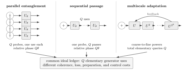
Parallel entanglement, repeated passage, and multiscale adaptive estimation can all accumulate an ideal phase leverage proportional to the total number $Q$ of elementary generator uses. Their preparation, coherence-time, loss, and control requirements differ, but counting only simultaneous particles would compare unlike resources.

The Resource Ledger

A defensible scaling statement names every resource that changes across the family of experiments. Common entries are:

Resource	Questions to settle
channel uses	How many times does a probe interrogate the unknown channel?
generator width	What eigenvalue range is available per use, in physical units?
probe number	Prepared, incident, interacting, detected, or accepted probes?
energy	Mean, maximum, or sector-resolved energy, and where is the zero chosen?
time	Interrogation, state preparation, reset, dead time, and total duration?
prior information	What interval or distribution localizes the parameter before sensing?
success probability	Are failures and discarded outcomes charged to the protocol?
controls	Are reference beams, ancillas, feedback, nonlinear interactions, and error correction free?
noise exposure	Does loss or decoherence grow with particle number, pass count, or duration?

For a bounded elementary generator, query count is often the cleanest theoretical resource. In a real sensor, time, energy through the sample, and damage may be more relevant. There need not be one scalar that captures every engineering constraint.

Block size versus total uses

Suppose each round uses an $N$-probe entangled block and there are $\nu$ independent rounds. The total number of elementary channel uses is

$$Q = \nu N.$$

The ideal local bound is

$$\Delta\theta \ge \frac{1}{N\sqrt\nu} = \frac{1}{\sqrt{QN}}.$$

At fixed $Q$, increasing the coherent block size improves this local bound, with the formal extreme $N=Q$ giving $1/Q$. But then $\nu=1$, outside the usual repeated-sample regime used to justify efficient local estimators. Global phase-estimation strategies distribute the same budget across different interrogation powers to obtain both range and resolution.

Energy constraints require care

For an unbounded generator such as photon number, a mean-energy constraint does not bound the variance. A state with a tiny amplitude on a very high-energy component can have a large QFI at fixed mean energy. This is not automatically a useful sub-Heisenberg sensor: its likelihood can have rare, fine features, poor global risk, and strong dependence on prior localization.

Maximum energy, total generator action, Bayesian average error, or a finite-difference bound can close different loopholes. The correct choice is part of the physical task, not a cosmetic normalization.

Local Sensitivity Is Not Global Accuracy

The QFI describes infinitesimal distinguishability around a specified $\theta$. A phase is periodic, so a global estimator should use a periodic loss such as

$$C(\widehat\theta-\theta) = 4\sin^2 \left( \frac{ \widehat\theta-\theta }{2} \right),$$

or explicitly declare how phase wraps are unwrapped. Ordinary squared error is suitable only after a branch convention and a sufficiently narrow range have been fixed.

A fixed-budget covariant solution

Let the generator have integer eigenvalues $n=0,1,\ldots,Q$, and take a uniform prior over one phase period. The sine state

$$|\psi_Q\rangle = \sqrt{ \frac{2}{Q+2} } \sum_{n=0}^{Q} \sin \left[ \frac{(n+1)\pi}{Q+2} \right] |n\rangle$$

with the canonical covariant phase measurement minimizes the average periodic cost in this model. Its first circular moment is

$$\left| \left\langle e^{i(\widehat\theta-\theta)} \right\rangle \right| = \cos \left( \frac{\pi}{Q+2} \right).$$

The Holevo phase variance is therefore

$$V_H = \tan^2 \left( \frac{\pi}{Q+2} \right) \sim \frac{\pi^2}{Q^2}.$$

This is a global Heisenberg-scaling result, but its constant differs from the unit-prefactor local QFI expression. The difference is not a contradiction: the tasks and risks differ.

Prior information is a resource

If the prior width already shrinks as $1/N$, a GHZ fringe can be confined to one branch and the local calculation becomes operational. If that prior was obtained from additional probes, those probes belong in the ledger. If it comes from stable external knowledge, the comparison must grant the same knowledge to the benchmark.

A robust protocol often uses a small fraction of its budget for coarse localization and the rest for fine estimation. Multiscale adaptive schemes make this explicit. Reporting only the finest interrogation power hides the cost of disambiguation.

Entanglement Is One Route, Not the Definition

For a linear collective generator and bounded local probes, multipartite entanglement is necessary to exceed the separable-state QFI bound $F_Q\le Nw^2$. It is therefore a resource for sub-SQL local sensitivity in that specific model.

Yet entanglement is neither a sufficient guarantee of useful metrology nor a universal prerequisite for $1/Q$ scaling. A GHZ state measured in the wrong basis carries no extracted Fisher information. A sequential protocol can achieve the same query scaling with one probe. Adaptive feedback, quantum memories, or coherent control can trade spatial entanglement for temporal coherence.

The operational question is not simply whether a state is entangled. It is whether the complete preparation–encoding–measurement–estimation protocol beats the best allowed comparator under the same resource and noise model.

Nonlinear Encodings and Apparent Super-Heisenberg Laws

Suppose the unknown coupling multiplies a $k$-body generator whose spectral width grows as $N^k$. The same generator-width argument permits

$$F_Q = O(N^{2k}), \qquad \Delta\theta = O(N^{-k})$$

for optimized entangled inputs. Product inputs can in some models achieve $O(N^{-(k-1/2)})$. Relative to particle number alone, these exponents are steeper than $N^{-1}$.

They do not violate the linear-query Heisenberg bound. The interaction graph contains a growing number of parameter-coupled terms, and the generator strength itself scales with $N$. Calling the result “super-Heisenberg” can be useful shorthand only when the nonlinear Hamiltonian and the charged resources are stated explicitly.

Preparation time is especially important near a quantum critical point. Susceptibility may grow rapidly with system size while the gap closes, so adiabatic preparation takes longer. A particle-only fit can then assign the benefit to criticality while omitting the time that generated the sensitive state. Similar care is required when control power or an externally supplied nonlinearity grows with $N$.

Independent Noise Usually Changes the Asymptote

Ideal $N^2$ QFI relies on coherence across generator eigenstates separated by $O(N)$. That same macroscopic separation often makes the probe fragile. Independent loss, dephasing, spontaneous emission, or imperfect visibility can suppress the coherence faster as the block grows.

For broad classes of independent, nonzero noise channels, channel-extension and purification bounds imply

$$F_Q^{(N)} \le c(\eta)N + o(N),$$

where $c(\eta)$ depends on the channel parameters. The asymptotic error then has SQL-like scaling,

$$\Delta\theta \gtrsim \frac{1}{ \sqrt{c(\eta)N} },$$

although a valuable constant-factor quantum gain may remain. This conclusion is powerful but not universal: correlated noise, non-Markovian dynamics, environment monitoring, noiseless subsystems, control, and quantum error correction define different channel classes.

Markovian dephasing example

Consider frequency estimation for total laboratory time $T$. Let one qubit interrogate for time $t$ while its coherence decays as $e^{-\gamma t}$. For $N$ product probes per round,

$$F_{Q,\mathrm{prod}}^{\mathrm{round}} = Nt^2e^{-2\gamma t}.$$

With approximately $T/t$ rounds,

$$F_{Q,\mathrm{prod}}^{\mathrm{tot}} = TNt e^{-2\gamma t}.$$

An $N$-qubit GHZ coherence decays as $e^{-N\gamma t}$, giving

$$F_{Q,\mathrm{GHZ}}^{\mathrm{tot}} = TN^2t e^{-2N\gamma t}.$$

The product strategy is optimized at $t=1/(2\gamma)$, whereas the GHZ strategy must shorten its interrogation to $t=1/(2N\gamma)$. Both maxima are

$$F_Q^{\mathrm{tot,max}} = \frac{TN}{2e\gamma}$$

under this idealized dephasing convention. The entangled state acquires phase faster but loses coherence faster by the same factor. Other noise models can leave a constant advantage, but this calculation shows why noiseless scaling cannot simply be extrapolated.

Loss and postselection

Postselecting no-loss events can restore high conditional visibility while making success exponentially rare. If $p_{\mathrm s}$ is independent of the unknown parameter and failures carry no information, the Fisher information per attempted round is

$$F_{\mathrm{attempt}} = p_{\mathrm s}F_{\mathrm{success}}.$$

For an intact $N$-particle branch with $p_{\mathrm s}\sim\eta^N$, the product $\eta^N N^2$ eventually decreases with $N$. Conditional precision alone is not an unconditional metrological gain.

When error correction can help

Quantum error correction can restore time-Heisenberg scaling under Markovian noise when the signal Hamiltonian has a component outside the real linear span generated by the identity, Lindblad operators, their adjoints, and their pairwise products. The result assumes resources such as sufficiently fast accurate control and suitable ancillas. If the signal lies entirely in that noise span, correcting the noise also erases the signal and the QFI remains at most linear in total time.

This signal-versus-noise condition is a precise exception, not a license to ignore decoherence. The controls, recovery cadence, ancilla quality, and uncorrectable errors must be included in an implementation claim.

Finite-Resource Crossovers

Asymptotic exponents do not determine which sensor is best at accessible resources. A useful schematic model is

$$(\Delta\theta)^2 = \frac{a}{N^2} + \frac{b}{N} + c,$$

where the terms may represent ideal coherent scaling, independent noise, and a technical floor. The logarithmic slope of the root error is

$$\alpha(N) = -\frac{d\log\Delta\theta}{d\log N}.$$

It can pass from nearly $1$ to $1/2$ and finally to $0$. A short data range can resemble any intermediate power. Fitting a straight line on a log–log plot without a mechanistic model, uncertainty on the exponent, or tests for correlated residuals does not establish asymptotic scaling.

Conversely, loss of the asymptotic exponent does not make quantum enhancement useless. A constant gain can reduce averaging time, sample exposure, or probe power substantially. The physically relevant comparison may be the minimum achievable error at a fixed finite budget, not the limiting slope.

From Bound to Demonstration

A convincing Heisenberg-scaling demonstration should report:

Item	Required evidence
estimand and risk	phase or physical parameter; local variance, circular risk, Bayesian MSE, or another loss
resource axis	channel uses, generator action, energy, time, or a justified vector of costs
comparator	best allowed independent or classical strategy under the same boundary
protocol accounting	preparation, coarse localization, adaptive passes, failures, and readout
operating range	prior width, dynamic range, phase-wrap rule, and calibration interval
noise model	loss, decoherence, drift, correlations, and how parameters were inferred
scaling evidence	multiple resource values, uncertainty on slope, crossover tests, and finite-$N$ performance
attainability	implemented measurement and estimator, not QFI alone

An experimental curve should distinguish predicted ideal scaling, measured pre-asymptotic behavior, and proven asymptotic bounds. These are different evidence classes. Claims, Hype, and Evidence Standards provides the broader reporting framework.

Common Mistakes

Counting carriers but not passes

One photon making $N$ passes uses the unknown channel $N$ times. Calling this an $N$-fold improvement at fixed resource because only one photon was present omits the central resource.

Treating local QFI as global mean-square error

A likelihood with $N$ fine fringes can have $F_Q=N^2$ and still leave the phase globally ambiguous. Prior localization or multiscale data must resolve the branch.

Calling every sub-SQL point Heisenberg scaling

A constant-factor gain below $1/\sqrt N$ has SQL exponent. Scaling is a claim about a family of resource values, not one point.

Ignoring attempts that failed

Heralding can improve the conditional data set while reducing the rate of successful data. Count all prepared probes and elapsed time unless the task genuinely makes failures free.

Using mean number and number variance interchangeably

For unbounded generators, fixed mean energy does not fix QFI. A local variance-based calculation and a global mean-resource bound answer different questions.

Calling nonlinear response a violation

If the parameter multiplies $O(N^k)$ interaction terms, particle number no longer measures total generator action. The stronger Hamiltonian belongs in the resource statement.

Assuming noise always forbids the scaling

Independent uncorrected noise often restores SQL-like asymptotics, but correlations, monitored environments, and error-corrected models can evade specific no-go assumptions. State the channel class.

Equating a bound with an achieved sensor

The QFI optimum may require a parameter-dependent or unavailable measurement. Preparation loss, readout noise, estimator bias, and calibration can erase an ideal advantage.

Exercises

1. Spectral-width bound

Let $G$ have eigenvalues in $[g_{\min},g_{\max}]$. Show that a pure-state unitary family generated by $G$ has $F_Q\le(g_{\max}-g_{\min})^2$, and identify a state that attains equality.

Solution

For a pure unitary family,

$$F_Q = 4(\Delta G)^2.$$

The variance of a random variable supported on an interval of width $g_{\max}-g_{\min}$ is at most one quarter of the squared width. Measurement of $G$ in any state produces such a random variable, so

$$(\Delta G)^2 \le \frac{(g_{\max}-g_{\min})^2}{4}.$$

Therefore $F_Q\le(g_{\max}-g_{\min})^2$. Equality is reached by

$$\frac{ |g_{\min}\rangle +e^{i\alpha}|g_{\max}\rangle }{\sqrt2},$$

which assigns equal probabilities to the interval endpoints.

2. GHZ fringe information and ambiguity

For $p_\pm=(1\pm\cos N\theta)/2$, compute the classical Fisher information. Then give two distinct phases in $[0,2\pi)$ that cannot be distinguished by this likelihood.

Solution

The derivatives are

$$\partial_\theta p_\pm = \mp\frac N2\sin(N\theta).$$

Thus

$$\begin{aligned} F_C &= \sum_{s=\pm} \frac{(\partial_\theta p_s)^2}{p_s} \\ &= \frac{N^2\sin^2(N\theta)}{4} \left( \frac1{p_+}+\frac1{p_-} \right) \\ &= N^2, \end{aligned}$$

with endpoint values obtained by continuity. Yet $\theta$ and $\theta+2\pi/N$ give identical probabilities. For example, $0$ and $2\pi/N$ are indistinguishable when $N>1$.

3. Parallel versus sequential queries

A single qubit in $|+\rangle$ experiences $U_\theta=e^{-i\theta\sigma_z/2}$ $m$ times coherently. Find its QFI with respect to $\theta$. Compare it with an $m$-qubit GHZ state and state the matched resource.

Solution

The total unitary is

$$U_\theta^m = e^{-im\theta\sigma_z/2}.$$

The effective generator is $m\sigma_z/2$, whose variance in $|+\rangle$ is $m^2/4$. Hence

$$F_Q = 4\frac{m^2}{4} = m^2.$$

An $m$-qubit GHZ state under one parallel use per qubit also has $F_Q=m^2$. The matched ideal resource is $m$ elementary channel uses or the same total generator exposure, not the number of simultaneously present carriers.

4. Optimize the dephasing time

Maximize

$$F(t) = TN^2t e^{-2N\gamma t}$$

over $t>0$. What scaling remains after optimization?

Solution

Differentiate the logarithm:

$$\frac{d}{dt}\log F = \frac1t-2N\gamma.$$

The maximum occurs at

$$t_* = \frac{1}{2N\gamma}.$$

Substitution gives

$$F(t_*) = \frac{TN}{2e\gamma}.$$

The optimized QFI is linear in $N$, so the root error scales as $N^{-1/2}$. The shorter optimal coherence interval removes the noiseless GHZ exponent.

5. Postselection ledger

An $N$-photon protocol has conditional Fisher information $N^2$ when every photon survives, and this happens with probability $\eta^N$. Find the Fisher information per attempt if failures carry no information. For fixed $0<\eta<1$, does increasing $N$ indefinitely help?

Solution

Including the success flag, and assuming its probability is parameter-independent, gives

$$F_{\mathrm{attempt}} = \eta^N N^2.$$

Its logarithm is

$$\log F_{\mathrm{attempt}} = N\log\eta+2\log N.$$

Because $\log\eta<0$, the linear negative term dominates the logarithm for large $N$. There is a finite optimum; arbitrarily large NOON states become worse per attempt in this simplified loss model.

6. Sine-state asymptotics

Starting from

$$V_H = \tan^2 \left( \frac{\pi}{Q+2} \right),$$

derive its large-$Q$ scaling and compare the root Holevo variance with the unit-prefactor local bound.

Solution

For small $x$, $\tan x=x+O(x^3)$. Therefore

$$V_H = \frac{\pi^2}{(Q+2)^2} + O(Q^{-4}),$$

and

$$\sqrt{V_H} \sim \frac{\pi}{Q}.$$

Both the global result and the local bound have exponent $-1$, but the global uniform-prior task carries a factor approaching $\pi$. Constants cannot be compared without matching the loss and prior.

7. Audit a nonlinear claim

A protocol estimates the coefficient of

$$H_\theta = \theta \sum_{i<j} \sigma_z^{(i)}\sigma_z^{(j)}$$

and reports $\Delta\theta\propto N^{-2}$. Explain why this does not by itself violate a linear-query Heisenberg limit.

Solution

The generator contains $N(N-1)/2=O(N^2)$ parameter-coupled pair terms, so its spectral width can grow quadratically with particle number. The experiment is not a family of $N$ uses of a fixed-strength one-body generator. Its resource ledger must include interaction terms, coupling strength, evolution time, and the cost of producing the nonlinear dynamics. Relative to total generator action, the apparent super-Heisenberg exponent need not exceed an inverse-resource law.

8. Design a scaling test

A sensor reports errors at $N=8,16,32,64$ and obtains a fitted slope $-0.93$. List four checks required before calling this evidence for Heisenberg scaling.

Solution

At minimum, the report should:

1. match channel uses, time, loss, prior information, and failed runs across all four values;
2. give uncertainty on the slope and test whether a crossover model fits as well as a single power law;
3. use an operational estimator and global loss, including phase-wrap failures rather than QFI alone;
4. show that state preparation, readout, calibration, and technical floors do not change systematically with $N$ in a way that creates the slope.

The four points may demonstrate useful finite-range behavior, but they do not alone prove an asymptotic theorem.

References

1. V. Giovannetti, S. Lloyd, and L. Maccone, “Quantum-enhanced measurements: Beating the standard quantum limit,” Science 306, 1330–1336 (2004), doi:10.1126/science.1104149.
2. V. Giovannetti, S. Lloyd, and L. Maccone, “Quantum metrology,” Physical Review Letters 96, 010401 (2006), doi:10.1103/PhysRevLett.96.010401.
3. V. Giovannetti, S. Lloyd, and L. Maccone, “Advances in quantum metrology,” Nature Photonics 5, 222–229 (2011), doi:10.1038/nphoton.2011.35.
4. S. L. Braunstein and C. M. Caves, “Statistical distance and the geometry of quantum states,” Physical Review Letters 72, 3439–3443 (1994), doi:10.1103/PhysRevLett.72.3439.
5. J. J. Bollinger, W. M. Itano, D. J. Wineland, and D. J. Heinzen, “Optimal frequency measurements with maximally correlated states,” Physical Review A 54, R4649–R4652 (1996), doi:10.1103/PhysRevA.54.R4649.
6. H. Lee, P. Kok, and J. P. Dowling, “A quantum Rosetta stone for interferometry,” Journal of Modern Optics 49, 2325–2338 (2002), doi:10.1080/0950034021000011536.
7. M. Zwierz, C. A. Pérez-Delgado, and P. Kok, “General optimality of the Heisenberg limit for quantum metrology,” Physical Review Letters 105, 180402 (2010), doi:10.1103/PhysRevLett.105.180402.
8. M. Zwierz, C. A. Pérez-Delgado, and P. Kok, “Ultimate limits to quantum metrology and the meaning of the Heisenberg limit,” Physical Review A 85, 042112 (2012), doi:10.1103/PhysRevA.85.042112.
9. M. J. W. Hall, D. W. Berry, M. Zwierz, and H. M. Wiseman, “Universality of the Heisenberg limit for estimates of random phase shifts,” Physical Review A 85, 041802(R) (2012), doi:10.1103/PhysRevA.85.041802.
10. D. W. Berry and H. M. Wiseman, “Optimal states and almost optimal adaptive measurements for quantum interferometry,” Physical Review Letters 85, 5098–5101 (2000), doi:10.1103/PhysRevLett.85.5098.
11. B. L. Higgins, D. W. Berry, S. D. Bartlett, H. M. Wiseman, and G. J. Pryde, “Entanglement-free Heisenberg-limited phase estimation,” Nature 450, 393–396 (2007), doi:10.1038/nature06257.
12. D. W. Berry et al., “How to perform the most accurate possible phase measurements,” Physical Review A 80, 052114 (2009), doi:10.1103/PhysRevA.80.052114.
13. M. Jarzyna and R. Demkowicz-Dobrzański, “True precision limits in quantum metrology,” New Journal of Physics 17, 013010 (2015), doi:10.1088/1367-2630/17/1/013010.
14. M. Tsang, “Ziv–Zakai error bounds for quantum parameter estimation,” Physical Review Letters 108, 230401 (2012), doi:10.1103/PhysRevLett.108.230401.
15. V. Giovannetti and L. Maccone, “Sub-Heisenberg estimation strategies are ineffective,” Physical Review Letters 108, 210404 (2012), doi:10.1103/PhysRevLett.108.210404.
16. S. Boixo, S. T. Flammia, C. M. Caves, and J. M. Geremia, “Generalized limits for single-parameter quantum estimation,” Physical Review Letters 98, 090401 (2007), doi:10.1103/PhysRevLett.98.090401.
17. S. Boixo et al., “Quantum-limited metrology with product states,” Physical Review A 77, 012317 (2008), doi:10.1103/PhysRevA.77.012317.
18. S. Boixo, A. Datta, M. J. Davis, S. T. Flammia, A. Shaji, and C. M. Caves, “Quantum metrology: Dynamics versus entanglement,” Physical Review Letters 101, 040403 (2008), doi:10.1103/PhysRevLett.101.040403.
19. M. J. W. Hall and H. M. Wiseman, “Does nonlinear metrology offer improved resolution? Answers from quantum information theory,” Physical Review X 2, 041006 (2012), doi:10.1103/PhysRevX.2.041006.
20. S. F. Huelga et al., “Improvement of frequency standards with quantum entanglement,” Physical Review Letters 79, 3865–3868 (1997), doi:10.1103/PhysRevLett.79.3865.
21. B. M. Escher, R. L. de Matos Filho, and L. Davidovich, “General framework for estimating the ultimate precision limit in noisy quantum-enhanced metrology,” Nature Physics 7, 406–411 (2011), doi:10.1038/nphys1958.
22. R. Demkowicz-Dobrzański, J. Kołodyński, and M. Guţă, “The elusive Heisenberg limit in quantum-enhanced metrology,” Nature Communications 3, 1063 (2012), doi:10.1038/ncomms2067.
23. R. Demkowicz-Dobrzański, M. Jarzyna, and J. Kołodyński, “Quantum limits in optical interferometry,” Progress in Optics 60, 345–435 (2015), doi:10.1016/bs.po.2015.02.003.
24. L. Pezzè, A. Smerzi, M. K. Oberthaler, R. Schmied, and P. Treutlein, “Quantum metrology with nonclassical states of atomic ensembles,” Reviews of Modern Physics 90, 035005 (2018), doi:10.1103/RevModPhys.90.035005.
25. S. Zhou, M. Zhang, J. Preskill, and L. Jiang, “Achieving the Heisenberg limit in quantum metrology using quantum error correction,” Nature Communications 9, 78 (2018), doi:10.1038/s41467-017-02510-3.
26. R. Demkowicz-Dobrzański, J. Czajkowski, and P. Sekatski, “Adaptive quantum metrology under general Markovian noise,” Physical Review X 7, 041009 (2017), doi:10.1103/PhysRevX.7.041009.
27. M. Kacprowicz, R. Demkowicz-Dobrzański, W. Wasilewski, K. Banaszek, and I. A. Walmsley, “Experimental quantum-enhanced estimation of a lossy phase shift,” Nature Photonics 4, 357–360 (2010), doi:10.1038/nphoton.2010.39.

Further Connections

• Quantum Measurement as Estimation defines the likelihood, estimator, risk, prior, nuisance model, and validation contract behind every scaling statement.
• Classical and Quantum Fisher Information derives the SLD QFI, pure-state generator formula, convexity, and measurement attainability used here.
• Cramér–Rao Bounds explains local unbiasedness, finite-sample limitations, Bayesian alternatives, and why a reciprocal QFI is not automatically an achieved error.
• Standard Quantum Limit develops the matched independent-probe benchmark and distinguishes constant gains from exponent changes.
• Squeezing explains how reduced noise becomes a metrological gain only after the reference, signal response, readout, and loss model are specified.
• Spin Squeezing shows how collective entanglement can yield an operational finite-$N$ gain without by itself proving Heisenberg scaling.
• Ramsey Interferometry shows explicitly how longer queries and GHZ fringes trade local information against coherence, cycle time, and global phase ambiguity.
• Mach–Zehnder Interferometry applies query counting and global-risk checks to NOON, Holland–Burnett, squeezed, and multipass optical probes under loss.
• Atomic Clocks compares CSS, GHZ, and squeezed probes after interrogation time, Markovian dephasing, oscillator phase wraps, and feedback are included.
• Noise and Decoherence in Metrology develops information-rate optimization, independent and correlated noise bounds, short-time scaling, control, monitoring, and error-corrected sensing.
• Quantum Channels and Noise supplies the channel language needed for noisy metrology bounds.
• Quantum Sensing develops decoherence, control, platform physics, and sensor implementations.
• Sensing Case Studies evaluates end-to-end evidence from representative experiments.
• Precision Measurement and Metrology connects these bounds to clocks, interferometers, field sensing, and real uncertainty budgets.