Quantum Measurement as Estimation

Measurement Produces Data; Estimation Produces an Answer

A quantum measurement does not normally reveal an unknown parameter directly. It produces a random classical outcome whose distribution depends on that parameter. Estimation is the subsequent statistical task of converting one or more outcomes into an estimate, interval, decision, or control action.

The basic chain is

$$\theta \longrightarrow \rho_\theta \longrightarrow x \sim p(x\mid\theta) \longrightarrow \widehat\theta(x).$$

Each arrow carries assumptions:

• $\theta$ must be a defined estimand with a domain and units;
• $\rho_\theta$ or the parameterized channel must model preparation, control, signal, and noise;
• the measurement must specify a POVM, instrument, or continuous record;
• $p(x\mid\theta)$ must include readout and selection rules;
• $\widehat\theta$ must be chosen for a declared loss or performance criterion.

This page is the canonical home for that end-to-end estimation contract. Quantum Sensing owns decoherence, backaction, noise spectroscopy, and platform examples. Fisher Information owns the generic classical metric, Classical and Quantum Fisher Information owns measurement optimization and the SLD quantum metric, and Standard Quantum Limit owns independent-probe scaling and matched-resource SQL claims.

Error Mitigation Overview applies this estimation contract to transformed noisy-circuit records, calibration-dependent estimators, conditional acceptance, covariance, and cost-qualified validation. Measurement Error Mitigation specializes that contract to calibrated terminal-response inversion, constrained or likelihood inference, unfolding, observable-dual correction, science and calibration covariance, structured scaling, and drift-qualified validation; this page retains general likelihood, loss, identifiability, uncertainty, and decision theory.

The Estimation Contract

A complete sensing problem should specify at least:

1. Estimand: the scalar, vector, waveform, field, or derived quantity to infer.
2. Parameter space: allowed values, periodicity, constraints, and prior range.
3. Probe and preparation: the initial state and controllable settings.
4. Encoding: the parameter-dependent state or channel, including noise.
5. Measurement: the POVM, instrument, detector response, and data retained.
6. Sampling design: repetitions, timing, adaptation, stopping, and postselection.
7. Nuisance parameters: calibration constants and unwanted unknowns.
8. Inference rule: estimator, posterior, test, classifier, or controller.
9. Loss or risk: what counts as an error and how errors are weighted.
10. Uncertainty statement: confidence region, credible region, or decision error.
11. Resource ledger: probe uses, energy, time, bandwidth, and failed runs.
12. Validation: calibration, predictive checks, held-out settings, and robustness.

Without these items, “the sensitivity is $\delta\theta$” is not yet a reproducible scientific statement.

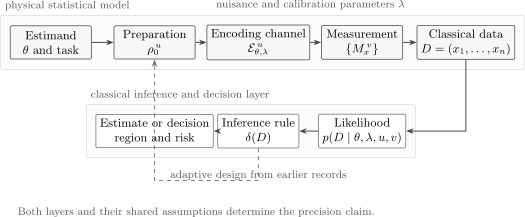
Quantum sensing has a physical statistical layer and a classical inference layer. Controls may be chosen in advance or adapted from earlier records. Nuisance parameters enter both layers. The final object is an estimate or decision with a quantified risk, not merely a measured observable.

Define the Estimand First

The estimand is the quantity the analysis promises to recover. It need not be an eigenvalue of an observable.

Task	Estimand	Typical data	Appropriate output
phase sensing	periodic phase $\theta\in[0,2\pi)$	binary outcomes or photon counts	circular estimate and interval
spectroscopy	frequency, detuning, or line center	counts versus interrogation setting	estimate with calibration and line-shape uncertainty
magnetometry	field amplitude, component, or waveform	spin readout records	scalar, vector, or time series
loss sensing	channel transmissivity $T$	click and no-click events	bounded estimate or one-sided interval
thermometry	temperature $T_{\mathrm{temp}}>0$	energies, populations, or trajectories	positive estimate and uncertainty
hypothesis testing	one of several states or channel models	measurement outcomes	decision and type-I/type-II errors

Several superficially similar targets can require different analyses. Estimating an instantaneous field value, a time average, a Fourier amplitude, and a model coupling are different tasks even when the same sensor produces the records.

Identifiability

A parameter is identifiable only if distinct allowed values lead to distinguishable data models. If

$$p(D\mid\theta,\lambda) = p(D\mid\theta',\lambda')$$

for every possible data set $D$, then the experiment cannot distinguish $(\theta,\lambda)$ from $(\theta',\lambda')$. More data from the same design do not cure structural non-identifiability. One needs an additional setting, calibration, prior restriction, or different measurement.

Identifiability is global. A model can also be locally blind when its derivative vanishes or when its Fisher matrix is singular at an operating point.

From a Quantum Model to a Likelihood

Let $u$ denote preparation and control settings, $\theta$ the target parameter, and $\lambda$ nuisance parameters. A general parameter-dependent output state can be written

$$\rho_{\theta,\lambda}^{\,u} = \mathcal E_{\theta,\lambda}^{\,u} \left( \rho_0^{\,u} \right),$$

where $\mathcal E_{\theta,\lambda}^{\,u}$ is a quantum channel. It may contain a unitary signal, dissipation, loss, environmental coupling, control error, or all of them.

For a POVM $\{M_x^{\,v}\}$ selected by measurement setting $v$,

$$M_x^{\,v}\succeq0, \qquad \sum_x M_x^{\,v}=I,$$

the Born rule gives the likelihood for one outcome:

$$p(x\mid\theta,\lambda,u,v) = \operatorname{Tr} \left[ M_x^{\,v} \rho_{\theta,\lambda}^{\,u} \right].$$

Once the state, channel, and POVM are fixed, this is an ordinary classical statistical model. Quantum theory constrains which likelihoods can be generated and which measurements are physically available; the estimator itself acts on classical data.

Measurement instruments and sequential data

A POVM gives outcome probabilities but not the conditional state required for later measurements. A quantum instrument $\{\mathcal I_x\}$ supplies both:

$$p(x\mid\rho) = \operatorname{Tr} \left[ \mathcal I_x(\rho) \right],$$ $$\rho_x = \frac{ \mathcal I_x(\rho) }{ p(x\mid\rho) }.$$

Sequential likelihoods depend on these state updates. If the next control depends on the observed history $x_{<k}=(x_1,\ldots,x_{k-1})$, then

$$\begin{aligned} p(x_{1:n}\mid\theta) = \prod_{k=1}^{n} p\left( x_k \middle| x_{<k}, \theta, u_k(x_{<k}) \right). \end{aligned}$$

Adaptive data are not identically distributed, but they still have a well-defined likelihood when the policy is specified. Ignoring the conditioning can double-count information or assign the wrong uncertainty.

Detector and Readout Models

The ideal POVM outcome $x$ may not equal the recorded symbol $y$. A classical readout channel $C(y\mid x)$ produces

$$q(y\mid\theta) = \sum_x C(y\mid x) p(x\mid\theta).$$

For a binary detector with false-positive probability $\alpha$ and false-negative probability $\beta$,

$$\begin{aligned} q(1\mid\theta) ={}& (1-\beta) p(1\mid\theta) \\ &+ \alpha \left[ 1-p(1\mid\theta) \right]. \end{aligned}$$

The analysis should fit or otherwise use $q$, not pretend the observed counts came from $p$. Algebraically inverting a confusion matrix can create negative corrected frequencies and unstable uncertainties. A forward likelihood naturally enforces probability constraints and propagates calibration uncertainty in $\alpha$ and $\beta$.

Loss and postselection are also part of the outcome model. A no-click event may carry information and cannot be discarded merely because it is inconvenient. If acceptance depends on $\theta$, conditioning only on accepted runs changes the likelihood and can bias the estimate.

Encoding Models

Unitary encoding

For a scalar phase,

$$\rho_\theta = e^{-i\theta G} \rho_0 e^{i\theta G},$$

where $G$ is the generator. The parameter may include a physical coupling and time, such as

$$\theta = \gamma BT.$$

Estimating $B$, $\gamma$, or $T$ is not the same task unless the other factors are known. Calibration uncertainty in $\gamma$ or $T$ becomes a nuisance parameter.

Channel encoding

Many targets change a channel rather than a closed-system phase:

$$\rho_\theta = \mathcal E_\theta(\rho_0).$$

Examples include transmissivity, dephasing rate, relaxation time, temperature-dependent dissipation, and an unknown force acting during open evolution. Ancillas and controls may improve channel discrimination, but the output likelihood must still include every retained mode and loss boundary.

Waveform encoding

A time-dependent signal $\theta(t)$ may enter a Hamiltonian

$$H(t) = H_0 + \theta(t)G.$$

The estimand might be the entire waveform, a filtered component, or coefficients in a basis expansion,

$$\theta(t) = \sum_{j=1}^{m} c_j f_j(t).$$

An infinite-dimensional waveform cannot be recovered from finite data without smoothness, bandwidth, sparsity, prior, or model assumptions. The reported resolution is therefore a property of both the sensor and the function class.

Estimators, Decisions, and Loss

An estimator is a function of the observed data:

$$\widehat\theta = \delta(D).$$

There is no universally best estimator independent of the loss, parameter range, and sampling model.

Frequentist risk

For loss $L(\widehat\theta,\theta)$, the frequentist risk is

$$R(\theta,\delta) = \mathbb E_\theta \left[ L( \delta(D), \theta ) \right].$$

With squared-error loss,

$$L( \widehat\theta,\theta ) = ( \widehat\theta-\theta )^2,$$

the risk is mean-square error. If

$$b(\theta) = \mathbb E_\theta[ \widehat\theta ] - \theta$$

is the bias, then

$$\operatorname{MSE}_\theta( \widehat\theta ) = \operatorname{Var}_\theta( \widehat\theta ) + b(\theta)^2.$$

A low-variance but strongly biased estimator may be worse than a noisier unbiased one.

Likelihood methods

The maximum-likelihood estimator is

$$\widehat\theta_{\mathrm{ML}} \in \operatorname*{arg\,max}_{\theta} p(D\mid\theta).$$

MLEs are often asymptotically efficient in regular identifiable models, but they can be biased at finite sample size, nonunique in periodic models, and pinned to boundaries. A likelihood value is not by itself a confidence probability for $\theta$.

Bayesian methods

Given a prior density $\pi(\theta)$,

$$\pi(\theta\mid D) = \frac{ p(D\mid\theta)\pi(\theta) }{ \int p(D\mid\vartheta) \pi(\vartheta) d\vartheta }.$$

A Bayes action minimizes posterior expected loss:

$$\widehat\theta_{\mathrm{B}} \in \operatorname*{arg\,min}_{a} \int L(a,\theta) \pi(\theta\mid D) d\theta.$$

For a real scalar, squared loss gives the posterior mean, absolute loss gives a posterior median, and zero–one loss in a discrete problem gives a maximum-posterior-probability decision. The prior is part of the model and should be justified, varied in a robustness analysis, and kept distinct from calibration data.

Minimax and hypothesis testing

A minimax rule controls worst-case risk,

$$\inf_\delta \sup_{\theta\in\Theta} R(\theta,\delta).$$

In hypothesis testing, the output is a decision rather than a point estimate. Performance is described by type-I and type-II errors, receiver-operating curves, or a cost-weighted decision risk. Estimation and testing can use the same measurement data but answer different questions.

Choose a Loss That Respects the Parameter

Ordinary squared error is inappropriate for every parameter space.

For a phase $\theta\in[0,2\pi)$, values near $0$ and $2\pi$ are close. A circular loss such as

$$L_{\mathrm{circ}} \left( \widehat\theta,\theta \right) = 4 \sin^2 \left( \frac{ \widehat\theta-\theta }{2} \right)$$

respects periodicity.

For a vector parameter, a weighted quadratic loss

$$L = ( \widehat{\boldsymbol\theta} - \boldsymbol\theta )^{\mathsf T} W ( \widehat{\boldsymbol\theta} - \boldsymbol\theta )$$

states which combinations matter. The units and scale in $W$ are substantive choices, not mathematical decoration.

For rare-event detection, missing a true signal and raising a false alarm may have very different costs. A credible sensing claim identifies the decision loss actually relevant to the application.

Local Information Versus Global Estimation

Classical and Quantum Fisher Information describes local curvature of a measured likelihood and its optimization over quantum measurements. Neither quantity alone solves a global estimation problem.

Consider a qubit prepared in

$$|+\rangle = \frac{ |0\rangle+|1\rangle }{\sqrt2}$$

and encoded by

$$U_\theta = e^{-i\theta\sigma_z/2}.$$

Measuring $X$ gives

$$p_X(+\mid\theta) = \frac{ 1+\cos\theta }{2}.$$

The data cannot distinguish $\theta$ from $-\theta$ or from $\theta+2\pi k$. This is a global ambiguity even where the local Fisher information is nonzero.

Measuring $Y$ instead gives

$$p_Y(+\mid\theta) = \frac{ 1+\sin\theta }{2},$$

which resolves the sign near $\theta=0$ but remains periodic globally. A known phase offset, several settings, an adaptive policy, or a prior interval can select a branch.

The quantum Cramér–Rao bound can be locally tight while global mean-square error remains large because of branch mistakes. Conversely, a globally robust measurement may sacrifice some local Fisher information to increase dynamic range.

Worked Example: Finite-Count Ramsey Estimation

Suppose a Ramsey-type experiment has contrast $C$, phase offset $\phi_0$, and plus-outcome probability

$$p_+( \theta,C,\phi_0 ) = \frac{ 1+ C\sin( \theta+\phi_0 ) }{2}.$$

From $n$ independent shots with $k$ plus outcomes,

$$p( k\mid \theta,C,\phi_0 ) = \binom nk p_+^k ( 1-p_+ )^{n-k}.$$

If $C$ and $\phi_0$ are known and the allowed phase lies on one monotone branch, an MLE is

$$\widehat\theta_{\mathrm{ML}} = \arcsin \left[ \frac{ 2k/n-1 }{C} \right] - \phi_0,$$

with boundary handling when finite counts put the argument outside $[-1,1]$.

If $C$ is also unknown, one setting identifies only the combination

$$C\sin( \theta+\phi_0 ).$$

Varying $\phi_0$, measuring another quadrature, or adding calibration data is required to separate phase from contrast. Reporting the known-$C$ error bar while estimating $C$ from the same finite data understates uncertainty.

Nuisance Parameters and Calibration

Write the full likelihood as

$$p(D\mid\theta,\boldsymbol\lambda),$$

where $\boldsymbol\lambda$ may include contrast, detection efficiency, background rate, phase offset, drift, temperature, coupling strength, or timing error.

For a regular local model with Fisher matrix

$$F = \begin{pmatrix} F_{\theta\theta} & F_{\theta\lambda} \\ F_{\lambda\theta} & F_{\lambda\lambda} \end{pmatrix},$$

the effective information about $\theta$ after allowing $\lambda$ to be unknown is the Schur complement

$$F_{\mathrm{eff}} = F_{\theta\theta} - F_{\theta\lambda} F_{\lambda\lambda}^{-1} F_{\lambda\theta},$$

when the inverse exists. Since the subtracted term is positive semidefinite, nuisance uncertainty cannot improve the local bound without additional information.

Calibration data can be included through a joint likelihood,

$$p( D_{\mathrm{science}}, D_{\mathrm{cal}} \mid \theta,\lambda ) = p( D_{\mathrm{science}} \mid \theta,\lambda ) p( D_{\mathrm{cal}} \mid \lambda ),$$

when the two data sets are conditionally independent. Treating an estimated calibration constant as exact discards its uncertainty.

Transmission and efficiency degeneracy

If a single photon is transmitted with probability $T$ and detected with efficiency $\eta$, an idealized click probability is

$$p_{\mathrm{click}} = \eta T.$$

From click/no-click data at one setting, only the product $\eta T$ is identifiable. Increasing the number of trials estimates that product more precisely but does not separate $T$ from $\eta$. A calibrated efficiency, a reference path, or another design is necessary.

Multiparameter Quantum Estimation

For several parameters, the classical Fisher information becomes a matrix and the estimator has a covariance matrix. Quantum optimization is subtler than maximizing each diagonal element independently.

Measurements optimal for different parameters may be incompatible. A quantum Fisher matrix can bound each local direction yet fail to be jointly attainable by one measurement on one copy. Collective measurements, weighted costs, Holevo-type bounds, and asymptotic protocols may be needed.

The practical design question is therefore not “What is the largest QFI?” but:

Which measurement and estimator minimize the declared joint risk under the available copies, controls, nuisance parameters, and compatibility constraints?

Classical and Quantum Fisher Information owns the SLD quantum Fisher matrix, compatibility criteria, and measurement optimization. Cramér–Rao Bounds owns the estimator-bound hierarchy, bias conditions, nuisance penalties, and global alternatives.

Continuous Records and Correlated Data

A continuously monitored system produces a time series rather than independent shots. The record might be a photocurrent, homodyne trace, sequence of quantum jumps, or thresholded event stream.

The likelihood is determined by the conditional dynamics. Schematically,

$$p( D_{0:T} \mid \theta ) = \prod_k p( dD_k \mid D_{<k}, \theta ).$$

A filter estimates the current conditional state or parameter using past data. A smoother may estimate a past signal using both earlier and later records. These are different causal tasks.

Autocorrelation reduces the effective information relative to an independent-sample count. Detector bandwidth, discretization, unobserved channels, and model mismatch enter the trajectory likelihood. Bayesian Quantum Measurement owns conditional state inference from records.

A state estimator reconstructs $\rho_t$ or its sufficient coordinates. A parameter estimator infers a fixed or time-varying model parameter. The two may be coupled, but they should not be conflated.

Experimental Design and Adaptation

Controls $u$ and measurement settings $v$ determine the likelihood. Design is therefore part of estimation.

Possible design criteria include:

• expected Fisher information near a nominal parameter;
• expected posterior variance or entropy;
• worst-case risk over an interval;
• probability of resolving competing hypotheses;
• robustness to nuisance parameters and drift;
• information gained per unit time, energy, or sample exposure.

An adaptive experiment chooses the next setting from earlier outcomes:

$$u_{k+1} = f( x_1,\ldots,x_k ).$$

This can keep an interferometer near a sensitive fringe, resolve phase branches, or concentrate data where competing models differ. The policy must be included in the likelihood and resource count.

Using the same data to choose a model, tune a stopping rule, and report an unadjusted interval can invalidate nominal coverage. Predeclared policies, sequential-analysis corrections, simulation-based calibration, or held-out validation data address different parts of this problem.

Uncertainty Is Part of the Result

A point estimate without uncertainty is incomplete.

Confidence regions

A $1-\alpha$ confidence procedure is designed so that, under repeated data generated at the true parameter,

$$\Pr_\theta[ \theta \in C(D) ] \ge 1-\alpha$$

over the declared model class. The probability statement concerns the procedure’s repeated-sampling coverage.

Credible regions

A Bayesian credible region $B(D)$ satisfies

$$\int_{B(D)} \pi( \theta\mid D ) d\theta = 1-\alpha.$$

This is a posterior probability statement conditional on the model and prior. A credible region need not have frequentist coverage, though some procedures can have both properties approximately or by design.

Systematic and model uncertainty

Repeated quantum shots reduce statistical uncertainty. They do not average away:

• a wrong Hamiltonian or channel model;
• an unknown calibration offset shared by every trial;
• drift outside the modeled stochastic process;
• selection bias;
• waveform components outside the assumed basis;
• detector nonlinearities absent from the likelihood.

Robustness checks should vary plausible model classes, nuisance priors, calibration assumptions, and data partitions. A narrow interval from a misspecified model is precise, not trustworthy.

Model Checking and Validation

Inference assumes the model can reproduce the data features relevant to the task. Useful checks include:

1. compare predicted and observed counts at settings not used to tune the model;
2. inspect residuals versus time, control setting, detector channel, and block;
3. test overdispersion and autocorrelation against the assumed sampling law;
4. inject known signals and recover them blind;
5. fit simulated data with known truth to measure bias and coverage;
6. compare nested or alternative noise models;
7. report sensitivity to calibration priors and truncation choices;
8. retain raw counts and metadata needed to reproduce the likelihood.

Good fit is necessary but not sufficient. Two nonidentifiable models can fit equally well while implying different physical parameters.

Reporting Checklist

A mature quantum-estimation result should report:

Layer	Minimum information
task	estimand, units, domain, local or global regime, and loss
quantum model	input state, parameterized channel, noise, and controls
measurement	POVM or record model, efficiency, bandwidth, and postselection
data	counts or traces, repetitions, timing, correlations, and failed runs
inference	likelihood, estimator or prior, optimizer, and stopping rule
nuisance handling	calibrated, jointly estimated, profiled, or marginalized
uncertainty	interval type, nominal level, coverage or prior dependence
resources	probes, incident energy, interactions, total time, and overhead
validation	injections, residuals, held-out tests, and model alternatives

The estimate should be reproducible from the reported model and data. The uncertainty should remain meaningful under the declared sampling or prior interpretation.

Common Mistakes

Calling an expectation value the estimate

$\langle M\rangle_\theta$ is a model prediction. A finite experiment produces data from which an estimator of $\theta$ is constructed.

Optimizing QFI without specifying an available measurement

QFI is a bound over measurements. It does not provide a detector, estimator, global branch rule, or finite-sample interval.

Ignoring non-identifiability

More repetitions sharpen identifiable combinations; they do not separate parameters that enter the likelihood only as a product or sum.

Treating calibration as exact

Estimated contrast, efficiency, phase offset, and background must carry uncertainty into the science result.

Reporting variance but not bias

Mean-square error contains both. A constant estimator can have zero variance and no inferential value.

Using linear loss for a periodic phase

An estimate near $2\pi$ is close to one near $0$, not far away.

Confusing state estimation with parameter estimation

Full tomography may be unnecessary for a scalar parameter, while a state filter does not automatically identify unknown dynamics.

Confusing metrological estimation with the phase-estimation algorithm

Quantum Phase Estimation is a coherent algorithm for estimating an eigenphase of a controlled unitary. It is not a synonym for every physical phase-sensing experiment.

Exercises

1. Find a phase ambiguity

A qubit phase experiment measures $X$ and has

$$p(+\mid\theta) = \frac{1+\cos\theta}{2}.$$

Name all parameter symmetries that leave the likelihood unchanged. Suggest one local remedy near $\theta=0$.

Solution

The likelihood is invariant under

$$\theta \mapsto -\theta$$

and under

$$\theta \mapsto \theta+2\pi k, \qquad k\in\mathbb Z.$$

Measuring $Y$ gives $(1+\sin\theta)/2$, which distinguishes the sign locally near zero. Equivalently, apply a known $\pi/2$ analysis phase before the $X$ measurement. Global $2\pi$ periodicity remains and requires a restricted interval, multiple scales, or a circular decision rule.

2. Include readout confusion

An ideal binary model has $p(1\mid\theta)=\theta$, with $0\le\theta\le1$. The detector has false-positive probability $\alpha=0.02$ and false-negative probability $\beta=0.08$. Find the observed success probability $q(1\mid\theta)$.

Solution

The observed one can arise from a correctly detected ideal one or a false positive:

$$\begin{aligned} q(1\mid\theta) &= (1-\beta)\theta + \alpha(1-\theta) \\ &= 0.92\theta + 0.02 - 0.02\theta \\ &= 0.02+0.90\theta. \end{aligned}$$

Fitting the ideal model directly to observed frequencies would produce a biased estimate of $\theta$.

3. Bayesian Bernoulli update

For $k$ successes in $n$ Bernoulli trials with success probability $\theta$, use a uniform prior on $[0,1]$. Find the posterior distribution and the Bayes estimator under squared-error loss.

Solution

The likelihood is proportional to

$$\theta^k (1-\theta)^{n-k}.$$

Multiplying by the uniform prior gives

$$\theta\mid D \sim \operatorname{Beta} \left( k+1, n-k+1 \right).$$

Squared-error loss selects the posterior mean:

$$\widehat\theta_{\mathrm B} = \frac{k+1}{n+2}.$$

This differs from the MLE $k/n$ and is generally biased in the frequentist sense at finite $n$.

4. Use circular loss

Two equally probable posterior phase values are $\epsilon$ and $2\pi-\epsilon$, with small $\epsilon>0$. What does an ordinary linear posterior mean give? What circular estimate is physically sensible?

Solution

Treating the interval as a line gives

$$\frac{ \epsilon+ (2\pi-\epsilon) }{2} = \pi,$$

which lies opposite both probable phases.

On the circle, both values lie near zero. Their unit phasors are complex conjugates with positive real part, so the circular mean direction is

$$\widehat\theta_{\mathrm{circ}} = 0 \pmod{2\pi}.$$

The loss and estimator must respect periodic geometry.

5. Decompose mean-square error

An estimator has bias $b=0.03$ and standard deviation $0.04$ in the parameter’s units. Find its mean-square error and root-mean-square error.

Solution

The variance is $0.04^2=0.0016$ and squared bias is $0.03^2=0.0009$. Therefore

$$\operatorname{MSE} = 0.0016+0.0009 = 0.0025,$$

and

$$\operatorname{RMSE} = \sqrt{0.0025} = 0.05.$$

6. Nuisance-parameter penalty

A two-parameter Fisher matrix is

$$F = \begin{pmatrix} 100&30\\ 30&25 \end{pmatrix},$$

where the first parameter is the target. Find the effective information when the second parameter is unknown.

Solution

The Schur complement is

$$\begin{aligned} F_{\mathrm{eff}} &= 100 - 30 \frac{1}{25} 30 \\ &= 100-36 \\ &= 64. \end{aligned}$$

The local variance bound is therefore $1/64$ rather than the misleading known-nuisance value $1/100$ for one use of this total Fisher matrix.

7. Diagnose transmission non-identifiability

A click probability is $p_{\mathrm{click}}=\eta T$. Alice observes enough data to determine $p_{\mathrm{click}}=0.42$ almost exactly. List three pairs $(\eta,T)$ consistent with the result and name one way to identify $T$.

Solution

Examples include

$$(\eta,T) \in \{ (0.6,0.7), (0.7,0.6), (0.84,0.5) \}.$$

All produce $0.42$. Alice can identify $T$ by independently calibrating $\eta$, adding a reference measurement with known transmission, or changing the design so $\eta$ and $T$ affect different recorded statistics.

8. Factor an adaptive likelihood

The first binary measurement uses setting $u_1$. If $x_1=1$, the second setting is $u_A$; otherwise it is $u_B$. Write the two-step likelihood.

Solution

The joint likelihood is

$$\begin{aligned} p( x_1,x_2 \mid \theta ) ={}& p( x_1 \mid \theta,u_1 ) \\ &\times p( x_2 \mid x_1,\theta,u_2(x_1) ), \end{aligned}$$

where

$$u_2(x_1) = \begin{cases} u_A,&x_1=1,\\ u_B,&x_1=0. \end{cases}$$

The second factor cannot be replaced by an unconditional identical-trial distribution because its setting and input state may depend on $x_1$.

9. Normalize an instrument branch

A quantum instrument maps $\rho$ to a subnormalized operator $\mathcal I_x(\rho)$ with trace $0.12$. What is the probability of $x$, and what state enters the next conditional step?

Solution

The outcome probability is

$$p(x\mid\rho) = \operatorname{Tr} \left[ \mathcal I_x(\rho) \right] = 0.12.$$

The normalized conditional state is

$$\rho_x = \frac{ \mathcal I_x(\rho) }{ 0.12 }.$$

Using the subnormalized operator directly as a density operator would corrupt the next-step probabilities.

10. Audit a precision claim

A paper quotes a posterior standard deviation for a magnetic field but gives no prior range, calibration model, or held-out validation. State four questions that must be answered before interpreting the number.

Solution

Suitable questions include:

1. What prior distribution and parameterization were used, and how sensitive is the result to them?
2. Which calibration quantities were fixed, and what uncertainty do they have?
3. Does the likelihood include readout error, drift, correlation, and selection?
4. Do posterior predictive or held-out settings agree with the fitted model?
5. Is the quoted standard deviation meaningful for a multimodal or bounded posterior?
6. What probes, time, bandwidth, and failed runs define the resource boundary?

Any four address distinct missing parts of the estimation contract.

References

1. A. Wald, Statistical Decision Functions, Wiley (1950), doi:10.1002/9780470316511.
2. E. L. Lehmann and G. Casella, Theory of Point Estimation, 2nd ed., Springer (1998), doi:10.1007/b98854.
3. H. L. Van Trees and K. L. Bell, Bayesian Bounds for Parameter Estimation and Nonlinear Filtering/Tracking, Wiley-IEEE Press (2007), doi:10.1002/0470120967.
4. C. W. Helstrom, Quantum Detection and Estimation Theory, Academic Press (1976), doi:10.1016/C2013-0-10310-8.
5. A. S. Holevo, Probabilistic and Statistical Aspects of Quantum Theory, 2nd ed., Edizioni della Normale (2011), doi:10.1007/978-88-7642-378-9.
6. S. L. Braunstein and C. M. Caves, “Statistical distance and the geometry of quantum states,” Physical Review Letters 72, 3439–3443 (1994), doi:10.1103/PhysRevLett.72.3439.
7. A. Fujiwara and H. Nagaoka, “Quantum Fisher metric and estimation for pure state models,” Physics Letters A 201, 119–124 (1995), doi:10.1016/0375-9601(95)00327-J.
8. R. D. Gill and S. Massar, “State estimation for large ensembles,” Physical Review A 61, 042312 (2000), doi:10.1103/PhysRevA.61.042312.
9. O. E. Barndorff-Nielsen, R. D. Gill, and P. E. Jupp, “On quantum statistical inference,” Journal of the Royal Statistical Society: Series B 65, 775–816 (2003), doi:10.1111/1467-9868.00415.
10. M. Hayashi, Asymptotic Theory of Quantum Statistical Inference: Selected Papers, World Scientific (2005), doi:10.1142/5605.
11. M. G. A. Paris, “Quantum estimation for quantum technology,” International Journal of Quantum Information 7, 125–137 (2009), doi:10.1142/S0219749909004839.
12. V. Giovannetti, S. Lloyd, and L. Maccone, “Advances in quantum metrology,” Nature Photonics 5, 222–229 (2011), doi:10.1038/nphoton.2011.35.
13. M. Tsang, H. M. Wiseman, and C. M. Caves, “Fundamental quantum limit to waveform estimation,” Physical Review Letters 106, 090401 (2011), doi:10.1103/PhysRevLett.106.090401.
14. S. Gammelmark and K. Mølmer, “Bayesian parameter inference from continuously monitored quantum systems,” Physical Review A 87, 032115 (2013), doi:10.1103/PhysRevA.87.032115.
15. C. Granade, C. Ferrie, N. Wiebe, and D. G. Cory, “Robust online Hamiltonian learning,” New Journal of Physics 14, 103013 (2012), doi:10.1088/1367-2630/14/10/103013.
16. D. W. Berry and H. M. Wiseman, “Optimal states and almost optimal adaptive measurements for quantum interferometry,” Physical Review Letters 85, 5098–5101 (2000), doi:10.1103/PhysRevLett.85.5098.

Further Connections

• Density Operators for Quantum Information supplies state families, classical–quantum registers, channels, and operational distance measures.
• POVMs: First Encounter introduces generalized outcome probabilities; instruments add conditional state updates.
• Bayes Rule owns the classical probability identity used in posterior inference.
• Classical and Quantum Fisher Information develops measurement-induced information, SLD formulas, geometry, and multiparameter compatibility.
• Cramér–Rao Bounds states the regularity and bias assumptions that turn those information metrics into variance or risk floors.
• Standard Quantum Limit derives the independent-probe benchmark after the estimation task and resource boundary are fixed.
• Heisenberg Scaling treats ideal inverse-resource precision, phase aliases, nonlinear encodings, and noise-aware scaling claims.
• Squeezing applies this estimation contract to reduced-noise observables, response-aware gains, calibration, and loss.
• Spin Squeezing applies it to collective-spin preparation, Ramsey response, entanglement certification, and clock evidence.
• Ramsey Interferometry develops the binary likelihood, working-point policy, phase aliases, adaptive design, and wall-clock resource accounting for Ramsey sensing.
• Mach–Zehnder Interferometry applies the contract to optical phase references, photon and sample resources, loss bounds, multipass queries, and postselection.
• Quantum Illumination applies the decision form of the contract to target absence versus presence, including Helstrom error, Chernoff exponents, receiver design, and matched classical benchmarks.
• Atomic Clocks extends the contract across correlated cycles, where a Bayesian state estimate and servo continually track a noisy oscillator.
• Precision Measurement and Metrology owns AMO implementations, calibration budgets, clocks, and interferometers.
• Claims, Hype, and Evidence Standards supplies the general claim-evidence-resource audit.