Spin Squeezing

Spin squeezing is the redistribution of fluctuations in a collective spin so that one transverse component is quieter than the coherent-spin reference. For spectroscopy and sensing, reduced noise is useful only if enough mean-spin length remains to convert a small rotation into a detectable signal. This is why two common squeezing parameters answer different questions:

• the Kitagawa–Ueda parameter asks whether a transverse spin variance is below coherent-spin noise;
• the Wineland parameter asks whether that variance, together with the signal response, enables a sub-standard-quantum-limit linear readout.

For $N$ effective spin-$1/2$ probes with a mean spin along $x$, the operational parameter is

$$\xi_R^2 = \frac{ N(\Delta J_\perp)^2 }{ |\langle\mathbf J\rangle|^2 }.$$

When the squeezed component is aligned with a Ramsey readout, one ideal trial has local phase variance

$$(\Delta\phi)^2 = \frac{\xi_R^2}{N}.$$

Thus $\xi_R^2<1$ means both a metrological gain over the matched coherent-spin state and, under the stated spin-$1/2$ model, a sufficient witness of multipartite entanglement. It does not establish a complete clock advantage: preparation time, atom loss, local-oscillator noise, detection noise, dynamic range, and accepted-shot rules still belong in the comparison.

This page is the canonical home for collective-spin squeezing parameters, generation mechanisms, Ramsey use, entanglement certification, and claim audits. Squeezing owns the cross-platform covariance and response framework. Spin Coherent States owns the general rotated highest-weight construction. Ramsey Interferometry for Quantum Estimation owns the binary likelihood, working-point control, phase aliases, and wall-clock information ledger. Ramsey Interferometry in Atomic, Molecular, and Optical Physics owns pulse dynamics and fringe formation, while Atomic Clocks and Optical Clocks own full instrument architectures and uncertainty budgets.

Collective Spin and the Coherent Reference

Take $N$ two-level systems and define dimensionless collective operators

$$J_k = \frac12 \sum_{i=1}^{N} \sigma_k^{(i)}, \qquad k\in\{x,y,z\}.$$

They obey

$$[J_i,J_j] = i\epsilon_{ijk}J_k.$$

Factors of $\hbar$ can be restored by replacing each $J_k$ with $\hbar J_k$. The collective language applies whenever the two modes of each probe can be treated as an effective qubit. They may be internal clock states, two momentum paths, two wells, or two interferometer arms. It does not imply that all physical spins or all couplings are literally identical.

The product state polarized along $+x$ is

$$|\mathrm{CSS}_x\rangle = |{+x}\rangle^{\otimes N}.$$

It lies in the symmetric total-spin sector $J=N/2$ and has

$$\begin{aligned} \langle J_x\rangle&=\frac N2, & \langle J_y\rangle&=\langle J_z\rangle=0,\\ (\Delta J_y)^2&=\frac N4, & (\Delta J_z)^2&=\frac N4. \end{aligned}$$

The $N/4$ transverse variance is quantum projection noise. It follows from adding $N$ independent binary fluctuations, not from technical uncertainty. The corresponding angular uncertainty is

$$\Delta\phi_{\mathrm{CSS}} = \frac{\Delta J_\perp}{|\langle\mathbf J\rangle|} = \frac1{\sqrt N}.$$

This is the independent-probe benchmark developed in Standard Quantum Limit. A fair squeezing claim compares against a coherent state with the same accepted atom number, interrogation, detection boundary, and repetition budget.

Transverse Covariance Geometry

Suppose the mean spin points along $x$. In the transverse $y$–$z$ plane define

$$V = \begin{pmatrix} (\Delta J_y)^2 & \operatorname{Cov}(J_y,J_z)\\ \operatorname{Cov}(J_y,J_z) & (\Delta J_z)^2 \end{pmatrix},$$

where

$$\operatorname{Cov}(A,B) = \frac12\langle AB+BA\rangle - \langle A\rangle\langle B\rangle.$$

A transverse component at angle $\vartheta$ is

$$J_\vartheta = J_y\cos\vartheta + J_z\sin\vartheta.$$

Its variance is the quadratic form

$$(\Delta J_\vartheta)^2 = \mathbf u_\vartheta^{\mathsf T} V \mathbf u_\vartheta, \qquad \mathbf u_\vartheta = \begin{pmatrix} \cos\vartheta\\ \sin\vartheta \end{pmatrix}.$$

The minimum and maximum transverse variances are the eigenvalues

$$V_\mp = \frac{V_{yy}+V_{zz}}2 \mp \frac12 \sqrt{ (V_{yy}-V_{zz})^2 + 4V_{yz}^2 }.$$

The principal-axis angle can be obtained from

$$\tan(2\vartheta_{\min}) = \frac{2V_{yz}}{V_{yy}-V_{zz}},$$

with the quadrant fixed by the covariance matrix rather than by the tangent alone. A nonlinear interaction often first creates a tilted ellipse. A collective rotation must then align its narrow axis with the component used by the estimator.

The Robertson–Schrödinger relation gives

$$V_{yy}V_{zz}-V_{yz}^2 \ge \frac14 |\langle J_x\rangle|^2.$$

Reducing $V_-$ therefore generally enlarges $V_+$, creates covariance, reduces the mean spin, or combines these effects. Spin squeezing redistributes quantum uncertainty; it does not remove the angular-momentum uncertainty relation.

Noise Squeezing and Metrological Squeezing

For $N$ spin-$1/2$ probes, the Kitagawa–Ueda parameter is

$$\xi_S^2 = \frac{4V_-}{N}.$$

It compares the narrowest transverse variance with the coherent-spin value $N/4$. Therefore

$$\xi_S^2<1$$

means transverse noise squeezing. This definition does not penalize loss of mean-spin length.

Define the Ramsey contrast or normalized spin length by

$$C = \frac{2|\langle\mathbf J\rangle|}{N}, \qquad 0\le C\le1.$$

The Wineland parameter is

$$\xi_R^2 = \frac{NV_-}{|\langle\mathbf J\rangle|^2} = \frac{\xi_S^2}{C^2}.$$

It is possible to have $\xi_S^2<1$ but $\xi_R^2\ge1$. The state is quieter than a coherent spin, yet its shortened mean spin provides too little signal slope for an improved linear Ramsey measurement.

For variance ratios, a positive quoted gain is conventionally

$$G_{\mathrm{dB}} = -10\log_{10}\xi_R^2.$$

Thus $\xi_R^2=0.25$ is $6.02\ \mathrm{dB}$ of metrological gain. The phase standard deviation improves only by

$$\xi_R = \sqrt{\xi_R^2} = 0.5.$$

Authors also use $\xi^2$, $\zeta^2$, or a signed decibel value for several inequivalent quantities. A reproducible result states the formula, reference, contrast treatment, and whether detection noise was included.

Ramsey Readout

Prepare a state with mean spin along $x$ and align the squeezed component with $J_y$. Let the unknown phase be encoded by

$$U_\phi = e^{-i\phi J_z}.$$

In the Heisenberg picture,

$$U_\phi^\dagger J_y U_\phi = J_y\cos\phi + J_x\sin\phi.$$

If $\langle J_y\rangle=0$, then near $\phi=0$,

$$\left. \frac{\partial\langle J_y\rangle_\phi}{\partial\phi} \right|_{\phi=0} = \langle J_x\rangle.$$

Error propagation gives

$$(\Delta\phi)^2 = \frac{(\Delta J_y)^2}{\langle J_x\rangle^2} = \frac{\xi_R^2}{N}.$$

After $\nu$ independent accepted repetitions,

$$(\Delta\phi)^2_\nu = \frac{\xi_R^2}{\nu N}.$$

The last two equations are local statements. They assume a calibrated midfringe, an approximately unbiased estimator, a known squeezing angle, and a phase prior narrow enough to avoid fringe aliases. Anti-squeezed noise can enter rapidly when the readout axis or local-oscillator phase is uncertain.

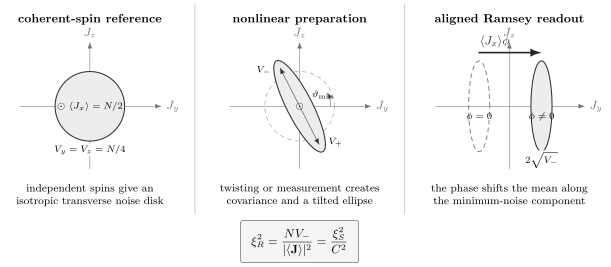
A coherent spin has equal transverse projection noise. A nonlinear or measurement-induced preparation creates a tilted noise ellipse, which is rotated so its narrow axis is read out after the signal phase. Metrological gain depends on both the narrow variance and the surviving mean-spin length.

For a clock transition of frequency $f_0$, Ramsey dark time $T$, cycle time $T_c$, and averaging duration $\tau$, the atom-noise-only estimate is

$$\sigma_y(\tau) \simeq \frac{\xi_R}{2\pi f_0T\sqrt N} \sqrt{\frac{T_c}{\tau}}.$$

This expression omits the Dick effect, local-oscillator phase noise, dead-time changes caused by squeezing preparation, state-detection errors, and systematic frequency shifts. Those omissions are why a measured $\xi_R^2<1$ is not by itself a complete clock demonstration.

Local Oscillator Mapping and Bloch-Sphere Curvature

Near a well-polarized state with total spin $J\simeq N/2$, define tangent-plane variables

$$X = \frac{J_y}{\sqrt J}, \qquad P = \frac{J_z}{\sqrt J}.$$

Because $[J_y,J_z]=iJ_x$,

$$[X,P] \simeq i$$

when $J_x\simeq J$. The coherent spin has

$$(\Delta X)^2 = (\Delta P)^2 = \frac12.$$

This Holstein–Primakoff regime explains why weak spin squeezing resembles oscillator quadrature squeezing. The approximation has a boundary: the spin phase space is a sphere, not an infinite plane. Strong nonlinear evolution can wrap or fold the distribution around the sphere. Then second moments and a linear $J_y$ readout may cease to capture the available phase information.

This oversqueezed regime can have poor $\xi_R^2$ even while the state has large quantum Fisher information. Nonlinear observables, parity, full distribution fitting, or an interaction-based echo may recover some of that information. It is therefore wrong to identify all metrologically useful many-body states with narrow Gaussian ellipses.

Entanglement and Fisher Information

For $N$ distinguishable spin-$1/2$ particles, every fully separable state obeys the collective-spin inequality

$$\xi_R^2 \ge 1.$$

Consequently,

$$\xi_R^2<1 \quad\Longrightarrow\quad \text{particle entanglement}.$$

The implication is one-way. GHZ states, twin-Fock states, Dicke states, and singlets may have vanishing mean spin, so the Wineland parameter is undefined or uninformative even when their entanglement and quantum Fisher information are large.

For a phase generated by $J_z$, the quantum Cramér–Rao bound and the available linear readout imply

$$F_Q[\rho,J_z] \ge \frac{N}{\xi_R^2}.$$

Thus $\xi_R^2<1$ certifies

$$F_Q[\rho,J_z]>N,$$

which is metrologically useful entanglement for that collective rotation. The reverse need not hold: $F_Q>N$ says that some measurement can beat the independent-probe bound locally, not that a first-moment spin readout does so.

Entanglement depth asks for the smallest number of particles that must be genuinely entangled in at least one cluster. A state is $k$-producible if it is a mixture of pure states whose entangled blocks contain at most $k$ particles. For $N$ qubits and a collective linear generator, such states satisfy

$$F_Q \le s k^2+r^2,$$

where

$$s = \left\lfloor\frac Nk\right\rfloor, \qquad r = N-sk.$$

Violating this bound rules out $k$-producibility. Spin-moment data can also be compared with the tighter polarization-dependent Sørensen–Mølmer curves. The often quoted estimate $1/\xi_R^2$ is not, by itself, an exact finite-$N$ entanglement depth. The witness must account for fluctuating atom number, inhomogeneous coupling, internal spin larger than $1/2$, and confidence intervals.

One-Axis Twisting

The canonical unitary mechanism is one-axis twisting,

$$H_{\mathrm{OAT}} = \hbar\chi J_z^2.$$

Starting from $|\mathrm{CSS}_x\rangle$, the evolution is

$$|\psi(t)\rangle = e^{-i\chi tJ_z^2} |\mathrm{CSS}_x\rangle.$$

Each $J_z$ sector acquires a phase proportional to $m_z^2$. On the tangent plane this produces a shear: slices with different $J_z$ rotate at different rates. The shear creates a nonzero $y$–$z$ covariance, so the minimum-noise axis is initially tilted. A linear spin rotation aligns that axis with the later readout.

In the ideal all-to-all collective model at large $N$,

$$\xi_{S,\min}^2 \propto N^{-2/3}, \qquad \chi t_{\mathrm{opt}} \propto N^{-2/3}.$$

This is stronger than a constant gain but weaker than ideal $1/N$ variance scaling. The asymptotic law does not survive automatically when $\chi$ changes with system size or when scattering, finite-range interactions, loss, and control overhead are included.

Past the optimum, the distribution bends around the Bloch sphere. The minimum linear variance eventually worsens even though non-Gaussian correlations continue to develop. An echo

$$U_{\mathrm{echo}} = U_{\mathrm{OAT}}^\dagger e^{-i\phi J_n} U_{\mathrm{OAT}}$$

can map a small phase into an amplified collective signal. Such interaction-based readout trades strict time reversal and control accuracy for relaxed detector resolution.

Two-Axis Countertwisting and Unstable Dynamics

With the mean spin along $x$, one form of two-axis countertwisting is

$$H_{\mathrm{TACT}} = \hbar\chi (J_yJ_z+J_zJ_y).$$

After a $45^\circ$ rotation in the transverse plane this is proportional to the difference of two squared spin components. One transverse direction is contracted while the orthogonal direction expands. In the local Gaussian regime the squeezing is approximately exponential, and the ideal collective model can reach

$$\xi_{min}^2 \propto \frac1N.$$

This is Heisenberg-like variance scaling under the specified collective-spin resource model. It is not a universal noisy scaling law. Exact two-axis interactions are harder to realize than one-axis twisting, so experiments may synthesize them with pulse sequences, continuous drives, Floquet engineering, or alternating interaction axes.

A related twist-and-turn model is

$$H_{\mathrm{TnT}} = \hbar\chi J_z^2 - \hbar\Omega J_x.$$

Near an unstable mean-field fixed point, fluctuations can separate rapidly along stable and unstable directions. This can generate strong squeezing or non-Gaussian states faster than simple shearing, but it also increases sensitivity to initialization, timing, and Hamiltonian calibration.

Measurement-Induced Squeezing

A quantum-nondemolition measurement can acquire information about one collective component without directly randomizing that same component. For an atomic spin $J_z$ coupled to an optical Stokes component $S_z$, a schematic interaction is

$$H_{\mathrm{QND}} = \hbar gS_zJ_z.$$

With a strongly polarized probe, an outgoing light quadrature carries an estimate of $J_z$. In a Gaussian model, combining prior variance $V_0$ with an independent measurement of equivalent variance $V_m$ gives conditional variance

$$\frac1{V_{\mathrm{cond}}} = \frac1{V_0} + \frac1{V_m}.$$

The optical measurement also causes spontaneous scattering, differential light shifts, coupling inhomogeneity, and backaction on the conjugate spin component. The useful quantity is therefore

$$\xi_R^2 = \frac{ NV_{\mathrm{cond}} }{ |\langle\mathbf J\rangle_{\mathrm{after}}|^2 },$$

not the conditional variance alone.

Without feedback, the conditional mean depends on the random measurement record. The ensemble of records can be broad even though each conditioned state is narrow. Real-time feedback rotates or displaces each conditioned state toward a common target and makes the preparation deterministic. A claim must say whether it concerns:

• a state conditioned on a recorded outcome;
• a postselected subset of outcomes;
• a feedback-stabilized deterministic state; or
• an unconditional density operator after the record is discarded.

These are operationally different resources, especially when success probability and latency are counted.

Physical Routes

Several mechanisms realize effective collective nonlinearities or measurements:

Route	Effective resource	Typical strength	Main liabilities
collisional dynamics in two-component condensates	state-dependent interactions produce $J_z^2$	direct one-axis twisting	particle loss, multimode dynamics, phase diffusion
cavity-mediated feedback	intracavity phase depends on population and feeds back on the spin	collective interaction and efficient readout	photon scattering, cavity inhomogeneity, technical detuning noise
dispersive QND probing	light records a collective population or spin component	conditional squeezing with simple observables	measurement backaction, optical loss, record conditioning
Rydberg dressing or blockade	programmable state-dependent interactions	finite-range or near-collective nonlinear evolution	decay, imperfect blockade, spatial nonuniformity
trapped-ion interactions	spin-dependent forces generate long-range couplings	precise unitary dynamics and echo readout	finite mode temperature, dephasing, system-size overhead
dipolar and spin-exchange dynamics	native many-body interactions redistribute collective noise	access to spin and spin-nematic observables	multilevel leakage, anisotropy, noncollective correlations

The same measured $\xi_R^2$ can emerge from very different states and noise channels. Platform comparisons should therefore include preparation time, accepted atom number, spatial mode, coherence, bandwidth, and readout method, not only the best decibel value.

Imperfections and Calibration

Contrast loss

If $\xi_S^2$ is held fixed while the contrast falls, then

$$\xi_R^2 = \frac{\xi_S^2}{C^2}$$

grows quadratically. For example, $6\ \mathrm{dB}$ of transverse variance reduction corresponds to $\xi_S^2\simeq0.25$. At contrast $C=0.5$, the Wineland parameter returns to approximately one.

Squeezing-angle error

Let $V_-$ and $V_+$ be the principal variances. A readout error $\delta$ sees

$$V_{\mathrm{read}} = V_-\cos^2\delta + V_+\sin^2\delta.$$

For small $\delta$,

$$V_{\mathrm{read}} \simeq V_- + \delta^2(V_+-V_-).$$

Stronger anti-squeezing therefore demands tighter phase control. Reporting only the narrow variance hides this vulnerability.

Detection noise

A calibrated linear detector often has

$$V_{\mathrm{obs}} = G^2V_{\mathrm{atom}} + V_{\mathrm{det}},$$

where $G$ is the atom-to-signal gain. Subtracting $V_{\mathrm{det}}$ can infer the atomic variance, but a sensor using that detector experiences $V_{\mathrm{obs}}$. Reports should distinguish raw performance from detection-noise-subtracted state characterization.

Inhomogeneous coupling

If probe $i$ couples with weight $w_i$, the measured operator is

$$J_z^{(w)} = \frac12 \sum_iw_i\sigma_z^{(i)}.$$

For an independent coherent reference,

$$\left(\Delta J_z^{(w)}\right)^2_{\mathrm{CSS}} = \frac14 \sum_iw_i^2,$$

not necessarily $N/4$. The signal slope involves $\sum_iw_i$ and may use a different spatial weighting. An effective atom number is meaningful only when its definition matches both noise and response.

Loss and fluctuating atom number

Random loss removes correlated particles, shortens the mean spin, and can add binomial noise. Fluctuating $N$ changes both the coherent reference and the mapping from population difference to phase. A robust analysis conditions on or models the measured $N$ for each shot, then propagates uncertainty in that calibration into $\xi_R^2$ and any entanglement-depth statement.

Decoherence during interrogation

Independent dephasing typically reduces

$$|\langle\mathbf J\rangle| \longrightarrow e^{-\Gamma T}|\langle\mathbf J\rangle|$$

while also modifying transverse covariances. Because the Wineland denominator contains the squared spin length, even modest decoherence can erase a state preparation gain. Common-mode noise may be rejected by a differential comparison, but that does not prove the same gain for two independent remote sensors.

Clocks and Many-Body Sensors

Spin squeezing is attractive for clocks because a collective population measurement is already the natural Ramsey output. Moderate squeezing can improve phase precision without requiring single-particle-resolved readout. The most credible evidence progresses through distinct levels:

1. a transverse variance below a calibrated coherent-spin reference;
2. a Wineland parameter below one after contrast and atom number are included;
3. a direct phase-estimation experiment below a matched independent-probe benchmark;
4. improved stability of a running clock or sensor with preparation, dead time, technical noise, and accepted data included.

These levels are not interchangeable. Early atomic-ensemble experiments established collective noise reduction and entanglement. Interacting condensates later demonstrated direct sub-SQL phase sensitivity. Cavity and QND methods produced stronger conditional or deterministic squeezing, and optical-clock experiments transferred squeezing to clock transitions and direct ensemble comparisons. Sensing Case Studies examines representative numerical claims and their experimental boundaries.

Many-body sensors extend the same logic beyond clocks. A collective spin may encode magnetic field, rotation, acceleration, interaction strength, or a spatially weighted signal. The best squeezed component must be aligned with the generator and measured mode. Local correlations that do not improve the chosen collective response may be scientifically interesting without improving that sensor.

Spin squeezing is also a many-body diagnostic. Collective first and second moments can witness entanglement in samples too large for tomography. This economy comes with limited resolution: different density operators can share the same moments, and failure to violate a squeezing inequality does not prove separability. Entanglement Witnesses develops the general witness logic.

Worked Example

Consider $N=10^4$ effective qubits. The coherent-spin transverse variance is

$$V_{\mathrm{CSS}} = \frac N4 = 2500.$$

Suppose tomography finds

$$V_- = 500, \qquad C = 0.80.$$

The noise-squeezing parameter is

$$\xi_S^2 = \frac{4V_-}{N} = 0.20.$$

The metrological parameter is

$$\xi_R^2 = \frac{0.20}{0.80^2} = 0.3125.$$

The corresponding gain is

$$G_{\mathrm{dB}} = -10\log_{10}(0.3125) \simeq 5.05\ \mathrm{dB}.$$

An ideal coherent state has one-shot local phase uncertainty $0.010\ \mathrm{rad}$. The squeezed state gives

$$\Delta\phi = \frac{\sqrt{0.3125}}{100} \simeq 5.59\times10^{-3}\ \mathrm{rad}.$$

The variance improved by a factor $3.2$, while the standard deviation improved by only $\sqrt{3.2}\simeq1.79$. A clock-level claim would still require cycle time, local-oscillator noise, and raw detector performance.

Claim Audit

Claim	Required evidence	What is not enough
transverse noise squeezing	calibrated $V_-<N/4$ for the declared measured mode	a narrow histogram without a coherent reference
metrological spin squeezing	$V_-$, contrast, atom number, response slope, and matched boundary	$\xi_S^2<1$ alone
particle entanglement	a valid separable-state inequality with model and confidence assumptions	reduced technical noise
entanglement depth	a stated $k$-producible bound including fluctuating $N$ and coupling inhomogeneity	rounding $1/\xi_R^2$ to an integer
sub-SQL phase sensing	direct estimator performance against a matched independent-probe experiment	inferred QFI without a realizable readout
improved clock or sensor	stability or risk with preparation, dead time, loss, calibration, and accepted trials included	a source-state decibel value
changed asymptotic scaling	a controlled resource family over increasing $N$ with noise and overhead tracked	one finite-$N$ gain point

Common Mistakes

• Using “spin squeezing” without stating which parameter is meant.
• Comparing $V_-$ with $N/4$ while the detector measures a weighted collective spin whose coherent variance is different.
• Ignoring the $C^{-2}$ contrast penalty in the Wineland parameter.
• Reporting a variance gain in decibels as the same numerical gain in standard deviation.
• Treating $\xi_R^2<1$ as necessary for entanglement rather than sufficient.
• Inferring exact entanglement depth as $1/\xi_R^2$ without the finite-$N$ witness curve.
• Calling conditional squeezing deterministic while discarding the measurement record or postselection probability.
• Subtracting detection noise for state characterization and then presenting the result as raw sensor performance.
• Assuming the ideal one-axis or two-axis scaling survives fixed decoherence, finite-range coupling, and preparation overhead.
• Treating clock stability, systematic accuracy, phase resolution, and entanglement depth as interchangeable metrics.

Exercises

1. Coherent-spin projection noise

For $|\mathrm{CSS}_x\rangle=|{+x}\rangle^{\otimes N}$, derive $\langle J_x\rangle=N/2$ and $(\Delta J_y)^2=(\Delta J_z)^2=N/4$.

Solution

For each probe,

$$\langle\sigma_x\rangle=1, \qquad \langle\sigma_y\rangle = \langle\sigma_z\rangle = 0.$$

Therefore

$$\langle J_x\rangle = \frac12\sum_i\langle\sigma_x^{(i)}\rangle = \frac N2.$$

Independence removes cross-covariances. Since $(\sigma_y^{(i)})^2=(\sigma_z^{(i)})^2=I$,

$$(\Delta J_y)^2 = \frac14\sum_i(\Delta\sigma_y^{(i)})^2 = \frac N4,$$

and similarly for $J_z$.

2. Find the squeezed axis

A transverse covariance matrix is

$$V = \begin{pmatrix} 10 & 6\\ 6 & 19 \end{pmatrix}.$$

Find its principal variances.

Solution

The eigenvalues are

$$V_\mp = \frac{29}2 \mp \frac12\sqrt{(-9)^2+4(6)^2}.$$

Because

$$\sqrt{81+144} = 15,$$

the principal variances are

$$V_-=7, \qquad V_+=22.$$

The off-diagonal covariance means neither laboratory axis is a principal axis; a rotation is required before readout.

3. Contrast can erase noise squeezing

A state has $\xi_S^2=0.16$. What minimum contrast is required for $\xi_R^2<1$? Evaluate $\xi_R^2$ at $C=0.30$.

Solution

Since

$$\xi_R^2 = \frac{\xi_S^2}{C^2},$$

metrological squeezing requires

$$C > \sqrt{0.16} = 0.40.$$

At $C=0.30$,

$$\xi_R^2 = \frac{0.16}{0.09} \simeq 1.78.$$

The transverse noise is squeezed, but the state does not beat the coherent linear-readout benchmark.

4. Ramsey slope

Show that a small rotation $e^{-i\phi J_z}$ maps a state with $\langle J_y\rangle=0$ to $\langle J_y\rangle_\phi\simeq\phi\langle J_x\rangle$. Identify the phase variance for a $J_y$ measurement.

Solution

The rotated observable is

$$J_y(\phi) = J_y\cos\phi + J_x\sin\phi.$$

Taking the expectation and expanding near zero gives

$$\langle J_y\rangle_\phi \simeq \phi\langle J_x\rangle.$$

Error propagation therefore yields

$$(\Delta\phi)^2 = \frac{(\Delta J_y)^2}{\langle J_x\rangle^2} = \frac{\xi_R^2}{N}$$

when $J_y$ is the aligned minimum-noise component.

5. Why one-axis twisting creates covariance

For $H=\hbar\chi J_z^2$, compute the Heisenberg equation for $J_y$ and give its leading behavior near a state polarized along $x$.

Solution

Using $\dot J_y=(i/\hbar)[H,J_y]$ and $[J_z,J_y]=-iJ_x$,

$$\dot J_y = \chi(J_zJ_x+J_xJ_z).$$

Near a strongly polarized state, replace $J_x$ by its mean value $J$:

$$\dot J_y \simeq 2\chi J J_z.$$

Thus different $J_z$ slices acquire different $J_y$ displacements. This is a shear in the transverse plane and creates $y$–$z$ covariance.

6. A Fisher-information depth bound

For $N=100$ and $\xi_R^2=0.20$, use $F_Q\ge N/\xi_R^2$. Can the state be four-producible?

Solution

The squeezing result implies

$$F_Q \ge \frac{100}{0.20} = 500.$$

For $k=4$,

$$s = \left\lfloor\frac{100}{4}\right\rfloor = 25, \qquad r=0.$$

Every four-producible state obeys

$$F_Q \le 25(4^2) = 400.$$

The observed lower bound exceeds 400, so the state is not four-producible and has entanglement depth at least five. The same argument does not certify depth six because the five-producible bound is 500 and the inferred QFI may equal that value.

7. Raw and inferred detector noise

A detector has gain $G=2$, observed variance $V_{\mathrm{obs}}=44$, and independently calibrated detector variance $V_{\mathrm{det}}=20$. Find the inferred atomic variance. Which variance belongs in a raw sensor claim?

Solution

From

$$V_{\mathrm{obs}} = G^2V_{\mathrm{atom}} + V_{\mathrm{det}},$$

we obtain

$$V_{\mathrm{atom}} = \frac{44-20}{4} = 6.$$

The value 6 characterizes the inferred atomic state under the detector model. The raw instrument experiences the full observed variance 44 in detector units, unless an additional protocol suppresses or calibrates that noise in the estimator.

8. Averaging-time gain

A squeezing protocol achieves $\xi_R^2=0.25$ without changing cycle time or other noise. By what factor does one-shot phase standard deviation improve? By what factor does the averaging time for a fixed variance decrease?

Solution

The standard-deviation ratio is

$$\xi_R = \sqrt{0.25} = 0.5.$$

The one-shot standard deviation is halved. Variance averages as $1/\nu$, so a factor of four fewer independent trials reaches the same target variance:

$$\frac{\tau_{\mathrm{sq}}}{\tau_{\mathrm{CSS}}} = \xi_R^2 = 0.25.$$

This conclusion fails if preparation increases cycle time or introduces additional technical noise.

References

1. D. J. Wineland, J. J. Bollinger, W. M. Itano, F. L. Moore, and D. J. Heinzen, “Spin squeezing and reduced quantum noise in spectroscopy,” Physical Review A 46, R6797–R6800 (1992), doi:10.1103/PhysRevA.46.R6797.
2. M. Kitagawa and M. Ueda, “Squeezed spin states,” Physical Review A 47, 5138–5143 (1993), doi:10.1103/PhysRevA.47.5138.
3. D. J. Wineland, J. J. Bollinger, W. M. Itano, and D. J. Heinzen, “Squeezed atomic states and projection noise in spectroscopy,” Physical Review A 50, 67–88 (1994), doi:10.1103/PhysRevA.50.67.
4. A. Sørensen, L.-M. Duan, J. I. Cirac, and P. Zoller, “Many-particle entanglement with Bose–Einstein condensates,” Nature 409, 63–66 (2001), doi:10.1038/35051038.
5. A. S. Sørensen and K. Mølmer, “Entanglement and extreme spin squeezing,” Physical Review Letters 86, 4431–4434 (2001), doi:10.1103/PhysRevLett.86.4431.
6. J. Ma, X. Wang, C. P. Sun, and F. Nori, “Quantum spin squeezing,” Physics Reports 509, 89–165 (2011), doi:10.1016/j.physrep.2011.08.003.
7. L. Pezzè, A. Smerzi, M. K. Oberthaler, R. Schmied, and P. Treutlein, “Quantum metrology with nonclassical states of atomic ensembles,” Reviews of Modern Physics 90, 035005 (2018), doi:10.1103/RevModPhys.90.035005.
8. G. Tóth and I. Apellaniz, “Quantum metrology from a quantum information science perspective,” Journal of Physics A 47, 424006 (2014), doi:10.1088/1751-8113/47/42/424006.
9. P. Hyllus, O. Gühne, and A. Smerzi, “Not all pure entangled states are useful for sub-shot-noise interferometry,” Physical Review A 82, 012337 (2010), doi:10.1103/PhysRevA.82.012337.
10. P. Hyllus, W. Laskowski, R. Krischek, C. Schwemmer, W. Wieczorek, H. Weinfurter, L. Pezzè, and A. Smerzi, “Fisher information and multiparticle entanglement,” Physical Review A 85, 022321 (2012), doi:10.1103/PhysRevA.85.022321.
11. G. Tóth, “Multipartite entanglement and high-precision metrology,” Physical Review A 85, 022322 (2012), doi:10.1103/PhysRevA.85.022322.
12. G. Tóth, C. Knapp, O. Gühne, and H. J. Briegel, “Optimal spin squeezing inequalities detect bound entanglement in spin models,” Physical Review Letters 99, 250405 (2007), doi:10.1103/PhysRevLett.99.250405.
13. J. Hald, J. L. Sørensen, C. Schori, and E. S. Polzik, “Spin squeezed atoms: A macroscopic entangled ensemble created by light,” Physical Review Letters 83, 1319–1322 (1999), doi:10.1103/PhysRevLett.83.1319.
14. A. Kuzmich, L. Mandel, and N. P. Bigelow, “Generation of spin squeezing via continuous quantum nondemolition measurement,” Physical Review Letters 85, 1594–1597 (2000), doi:10.1103/PhysRevLett.85.1594.
15. J. Appel, P. J. Windpassinger, D. Oblak, U. B. Hoff, N. Kjærgaard, and E. S. Polzik, “Mesoscopic atomic entanglement for precision measurements beyond the standard quantum limit,” Proceedings of the National Academy of Sciences 106, 10960–10965 (2009), doi:10.1073/pnas.0901550106.
16. I. D. Leroux, M. H. Schleier-Smith, and V. Vuletić, “Implementation of cavity squeezing of a collective atomic spin,” Physical Review Letters 104, 073602 (2010), doi:10.1103/PhysRevLett.104.073602.
17. C. Gross, T. Zibold, E. Nicklas, J. Estève, and M. K. Oberthaler, “Nonlinear atom interferometer surpasses classical precision limit,” Nature 464, 1165–1169 (2010), doi:10.1038/nature08919.
18. M. F. Riedel, P. Böhi, Y. Li, T. W. Hänsch, A. Sinatra, and P. Treutlein, “Atom-chip-based generation of entanglement for quantum metrology,” Nature 464, 1170–1173 (2010), doi:10.1038/nature08988.
19. Y. Li, Y. Castin, and A. Sinatra, “Optimum spin squeezing in Bose–Einstein condensates with particle losses,” Physical Review Letters 100, 210401 (2008), doi:10.1103/PhysRevLett.100.210401.
20. O. Hosten, N. J. Engelsen, R. Krishnakumar, and M. A. Kasevich, “Measurement noise 100 times lower than the quantum-projection limit using entangled atoms,” Nature 529, 505–508 (2016), doi:10.1038/nature16176.
21. K. C. Cox, G. P. Greve, J. M. Weiner, and J. K. Thompson, “Deterministic squeezed states with collective measurements and feedback,” Physical Review Letters 116, 093602 (2016), doi:10.1103/PhysRevLett.116.093602.
22. O. Hosten, R. Krishnakumar, N. J. Engelsen, and M. A. Kasevich, “Quantum phase magnification,” Science 352, 1552–1555 (2016), doi:10.1126/science.aaf3397.
23. E. Pedrozo-Peñafiel et al., “Entanglement on an optical atomic-clock transition,” Nature 588, 414–418 (2020), doi:10.1038/s41586-020-3006-1.
24. M. Schulte, C. Lisdat, P. O. Schmidt, U. Sterr, and K. Hammerer, “Prospects and challenges for squeezing-enhanced optical atomic clocks,” Nature Communications 11, 5955 (2020), doi:10.1038/s41467-020-19403-7.
25. W. J. Eckner et al., “Realizing spin squeezing with Rydberg interactions in an optical clock,” Nature 621, 734–739 (2023), doi:10.1038/s41586-023-06360-6.
26. J. M. Robinson et al., “Direct comparison of two spin-squeezed optical clock ensembles at the $10^{-17}$ level,” Nature Physics 20, 208–213 (2024), doi:10.1038/s41567-023-02310-1.

Further Connections

• Squeezing develops the platform-independent relation among covariance, reference noise, signal response, loss, and readout.
• Standard Quantum Limit derives the coherent-spin and independent-probe benchmark used here.
• Classical and Quantum Fisher Information explains the measurement-optimized information bound and why a linear spin readout need not attain it.
• Heisenberg Scaling separates finite-$N$ gain from an asymptotic inverse-resource law.
• Spin Coherent States supplies the rotated highest-weight geometry and transverse coherent noise.
• Ramsey Interferometry for Quantum Estimation develops the likelihood, Fisher information, phase aliases, adaptive settings, and duty-cycle accounting for the readout used here.
• Atomic Clocks tests spin-squeezing gain after preparation time, oscillator noise, dead time, phase wraps, feedback, and independent validation are included.
• Magnetometry applies spin squeezing to a specified magnetic-field mode and tests gain after bandwidth, volume, dynamic range, and wall time are matched.
• Gravimetry and Inertial Sensing follows squeezing through momentum-mode transfer, inertial phase encoding, readout, resource matching, and a calibrated acceleration or gravity estimate.
• Ramsey Interferometry derives the separated-pulse fringe and population readout used by clocks and qubit sensors.
• Atomic Clocks and Optical Clocks own complete clock cycles, oscillator noise, systematic shifts, and stability.
• Sensing Case Studies compares state-level, estimator-level, and running-instrument evidence.
• Entanglement Witnesses gives the general logic of observable bounds that all separable states must obey.
• Dephasing Channel develops the coherence loss that commonly limits collective-spin metrology.