Quantum Illumination

Quantum illumination is entanglement-assisted discrimination between two lossy, noisy channels: one describing an absent target and one describing a weakly reflecting target. A source prepares correlated signal–idler mode pairs. The signal interrogates a target region, the idler is retained, and a receiver jointly processes the collected return and retained idler to decide which channel acted.

Its best-known result is striking but narrow. For many independent low-brightness mode pairs, a weak specular reflector of known phase, and a bright thermal background, an ideal two-mode-squeezed transmitter with an optimum joint receiver has an error-probability exponent four times that of an optimum-reception coherent-state transmitter at the same transmitted signal energy. This factor of four is conventionally called a 6 dB error-exponent advantage. It can survive even when loss and noise make the received return–idler state separable.

That theorem does not establish a six-decibel improvement in received power, range, cross section, or arbitrary radar performance. It assumes a declared hypothesis pair, known mode matching, a particular background model, an ideal idler, and an optimum receiver. Unknown phase, speckle, range search, Doppler, clutter, receiver loss, idler storage, and wall-clock duty cycle can change or remove the advantage. Quantum illumination is therefore best understood as a precise result in quantum channel discrimination, not as a synonym for every sensor using correlated radiation.

Canonical Scope

This page owns the target-detection and receiver-comparison layer of quantum illumination:

• binary target absence versus presence as a quantum hypothesis test;
• the Gaussian signal, idler, return, and thermal-background model;
• Helstrom error, receiver-operating curves, and Chernoff exponents;
• the matched classical-state benchmark and the 3 dB and 6 dB regimes;
• optical-parametric-amplifier, phase-conjugate, sum-frequency-generation, correlation-to-displacement, coincidence, and digital receivers;
• idler loss, source impurity, unknown phase, fading, mode search, and information per experimental resource;
• the distinction between theorem, proof-of-principle experiment, and radar engineering claim.

Two-Mode Entanglement owns the state theory of two-mode squeezing. Parametric Down-Conversion owns optical pair generation and collection physics. Gaussian Channels owns general bosonic attenuation and noise channels. Quantum Measurement as Estimation owns the broader decision-theoretic contract. Those topics are used here only as needed to formulate the target-detection problem.

The Detection Contract

Before choosing a quantum source, define what constitutes a target and what constitutes an error.

Two hypotheses

For one matched temporal-frequency-spatial mode, let $\hat a_S$ denote the transmitted signal, $\hat a_I$ the retained idler, and $\hat a_R$ the collected return. A standard specular-target model is

$$\begin{aligned} H_0 &: \quad \hat a_R = \hat b_0, \\[3pt] H_1 &: \quad \hat a_R = \sqrt{\kappa}\,e^{i\phi}\hat a_S + \sqrt{1-\kappa}\,\hat b_1. \end{aligned}$$

Here $H_0$ means target absent, $H_1$ means target present, $\kappa\ll1$ is the round-trip transmissivity into the collected mode, and $\phi$ is the return phase. The bath modes are thermal and independent of the source. In the usual passive-signature convention, they are chosen so that the received background brightness is $N_B$ under either hypothesis:

$$\langle \hat b_0^\dagger\hat b_0\rangle=N_B, \qquad \langle \hat b_1^\dagger\hat b_1\rangle = \frac{N_B}{1-\kappa}.$$

Consequently,

$$\begin{aligned} \langle \hat a_R^\dagger\hat a_R\rangle_{H_0} &=N_B, \\ \langle \hat a_R^\dagger\hat a_R\rangle_{H_1} &=N_B+\kappa N_S, \end{aligned}$$

where $N_S=\langle\hat a_S^\dagger\hat a_S\rangle$ is signal photons per mode. This convention prevents an artificial detector from deciding between $H_0$ and $H_1$ merely because inserting the target changes the background level. A different physical background model is legitimate, but it defines a different discrimination problem and must be used for both quantum and classical systems.

Priors, costs, and errors

Let $\Pi_0$ and $\Pi_1$ be the receiver’s two decision operators, with $\Pi_0+\Pi_1=\mathbb I$. The false-alarm and miss probabilities are

$$P_{\mathrm{FA}} = \operatorname{Tr}(\Pi_1\rho_0), \qquad P_{\mathrm{M}} = \operatorname{Tr}(\Pi_0\rho_1).$$

For prior probabilities $\pi_0$ and $\pi_1$ and equal costs for the two error types, the Bayes error is

$$P_e = \pi_0P_{\mathrm{FA}} + \pi_1P_{\mathrm{M}}.$$

Equal priors are mathematically convenient, but many sensing systems operate at low target prevalence and impose a stringent false-alarm constraint. The appropriate output is then a receiver-operating characteristic or a Neyman–Pearson miss probability at fixed $P_{\mathrm{FA}}$, not only an equal-prior error number. Threshold tuning after seeing test data invalidates either comparison.

Many matched modes

A broadband pulse or observation interval contains many approximately orthogonal mode pairs. In the ideal independent-and-identically-distributed model,

$$\rho_j^{(M)} = \rho_j^{\otimes M}, \qquad j\in\{0,1\}.$$

For duration $T$ and usable bandwidth $W$, the order of magnitude is $M\sim TW$, up to real-mode versus complex-mode conventions and polarization factors. The transmitted photon budget is

$$N_{\mathrm{tx}}=MN_S, \qquad E_{\mathrm{tx}}=\hbar\omega MN_S$$

for a narrowband carrier. Reporting $N_S$ without $M$, or $M$ without source brightness, does not specify the exposure.

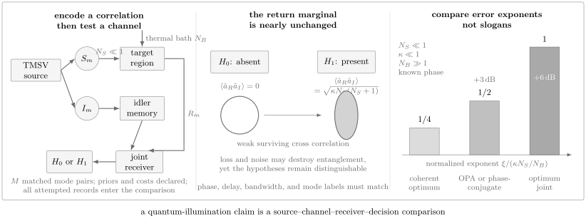
Quantum illumination places a correlated source, a noisy target channel, an idler memory, and a receiver inside one decision problem. The exponent ladder applies only in the stated low-brightness, weak-reflectivity, bright-background, known-phase regime. A receiver demonstration and a source demonstration are not by themselves a complete target-detection advantage.

The Gaussian Quantum-Illumination Source

Two-mode squeezed vacuum

The canonical Gaussian transmitter uses $M$ two-mode squeezed-vacuum pairs. For each pair,

$$\lvert\psi\rangle_{SI} = \sum_{n=0}^{\infty} \sqrt{\frac{N_S^n}{(N_S+1)^{n+1}}} \lvert n\rangle_S\lvert n\rangle_I.$$

Each marginal is thermal,

$$\langle \hat a_S^\dagger\hat a_S\rangle = \langle \hat a_I^\dagger\hat a_I\rangle =N_S,$$

but the pair has phase-sensitive cross correlation

$$\langle \hat a_S\hat a_I\rangle = \sqrt{N_S(N_S+1)}$$

in a convenient phase convention. A classical signal–idler state with a positive Glauber–Sudarshan representation obeys the Cauchy–Schwarz bound

$$\bigl\lvert \langle \hat a_S\hat a_I\rangle \bigr\rvert^2 \leq N_SN_I.$$

For equal signal and idler brightness $N_I=N_S$, a two-mode squeezed vacuum has correlation squared $N_S(N_S+1)$ rather than at most $N_S^2$. The relative gap is especially large when $N_S\ll1$. Quantum illumination encodes target presence in the weak remnant of this initially nonclassical correlation.

Covariance matrices under the hypotheses

Use quadratures with vacuum variance $1/2$ and define

$$\mathbf Z = \begin{pmatrix} 1&0\\ 0&-1 \end{pmatrix}.$$

For known phase $\phi=0$, the return–idler covariance matrices are

$$V_{RI}^{(0)} = \begin{pmatrix} (N_B+\tfrac12)\mathbb I_2 & 0\\ 0 & (N_S+\tfrac12)\mathbb I_2 \end{pmatrix}$$

and

$$V_{RI}^{(1)} = \begin{pmatrix} (N_B+\kappa N_S+\tfrac12)\mathbb I_2 & \sqrt{\kappa N_S(N_S+1)}\,\mathbf Z \\ \sqrt{\kappa N_S(N_S+1)}\,\mathbf Z & (N_S+\tfrac12)\mathbb I_2 \end{pmatrix}.$$

When $N_B\gg\kappa N_S$, the return marginal changes only slightly. The main signature available to a joint receiver is the off-diagonal block. Under $H_0$ it vanishes; under $H_1$ it is proportional to $\sqrt{\kappa N_S(N_S+1)}$.

Advantage after entanglement is gone

In this convention, the thermal-loss channel is entanglement breaking when $N_B\geq\kappa$. The returned mode and stored idler are then separable even under $H_1$. This does not make the two conditional states identical. The initial entangled source created a phase-sensitive correlation stronger than any equal-energy classical source could create; attenuation leaves a weak but measurable remnant of that correlation.

The operational resource statement is therefore:

Initial signal–idler entanglement enables a stronger transmitter correlation, while target detection uses distinguishability between the two final return–idler states.

It is misleading to say that entanglement itself travelled out and back intact. It is also unnecessary to identify one surviving correlation measure, such as discord, as the unique cause of the advantage. The performance claim is settled by a matched channel-discrimination bound.

Quantum Hypothesis Testing

Helstrom limit

For arbitrary priors, the minimum Bayes error over all two-outcome POVMs is

$$P_e^\star = \frac12 \left[ 1- \left\lVert \pi_1\rho_1^{(M)} - \pi_0\rho_0^{(M)} \right\rVert_1 \right].$$

For equal priors this becomes

$$P_e^\star = \frac12 \left[ 1- \frac12 \left\lVert \rho_1^{(M)}-\rho_0^{(M)} \right\rVert_1 \right].$$

The corresponding Helstrom measurement projects onto the positive and negative eigenspaces of $\pi_1\rho_1^{(M)}-\pi_0\rho_0^{(M)}$. This defines the optimum, but directly diagonalizing a many-mode mixed-state difference does not by itself give a practical optical receiver.

Quantum Chernoff exponent

For equal priors and independent copies, define

$$Q := \inf_{0\leq s\leq1} \operatorname{Tr} \left( \rho_0^s\rho_1^{1-s} \right), \qquad \xi_Q:=-\ln Q.$$

The quantum Chernoff bound is

$$P_e^\star(M) \leq \frac12Q^M = \frac12e^{-M\xi_Q}.$$

More importantly, the exponent is asymptotically exact:

$$\lim_{M\to\infty} -\frac1M\ln P_e^\star(M) = \xi_Q.$$

An exponent is not an exact finite-sample error probability. Prefactors, non-identical modes, calibration uncertainty, and threshold estimation matter before the asymptotic regime is reached.

The Error-Exponent Hierarchy

The standard asymptotic regime

The familiar comparison assumes

$$N_S\ll1, \qquad \kappa\ll1, \qquad N_B\gg1, \qquad M\gg1,$$

with known return phase and ideal mode matching. Let

$$\gamma := \frac{\kappa N_S}{N_B}.$$

For a coherent-state transmitter with optimum reception, the leading error exponent is

$$\xi_{\mathrm{coh}} \simeq \frac{\gamma}{4}, \qquad P_{e,\mathrm{coh}} \sim \frac12 \exp\!\left(-\frac{M\kappa N_S}{4N_B}\right).$$

This is not merely a comparison with direct detection. Coherent light is the canonical classical transmitter for the specified Gaussian channel, and it is paired here with optimum quantum reception. The original positive-$P$ analysis also bounds arbitrary classical signal–idler transmitters, but that general bound is looser than the exact coherent-state result. An experiment claiming the best classical benchmark must therefore state its allowed transmitter, idler, receiver, amplifier, and reference resources rather than infer that claim from a comparison with one convenient classical apparatus.

Structured pairwise quantum-illumination receivers such as ideal OPA and phase-conjugate receivers attain

$$\xi_{\mathrm{pair}} \simeq \frac{\gamma}{2}.$$

The optimum joint quantum receiver attains

$$\xi_{\mathrm{QI}} \simeq \gamma.$$

Thus

$$\frac{\xi_{\mathrm{pair}}}{\xi_{\mathrm{coh}}} \simeq2, \qquad \frac{\xi_{\mathrm{QI}}}{\xi_{\mathrm{coh}}} \simeq4.$$

Expressed in decibels,

$$10\log_{10}2\simeq3.01\ \mathrm{dB}, \qquad 10\log_{10}4\simeq6.02\ \mathrm{dB}.$$

The logarithm applies to a ratio of error exponents. It does not mean that $P_e$ itself is smaller by 6 dB. Because $P_e$ is exponential in $M$, a fourfold exponent can yield a much larger error-probability ratio after many modes. Conversely, outside the asymptotic assumptions there need not be a fourfold ratio at all.

Exact coherent-state expression

For the ideal known-phase Gaussian model, the coherent-state Chernoff exponent before the bright-background approximation is

$$\xi_{\mathrm{coh}} = \kappa N_S \left( \sqrt{N_B+1}-\sqrt{N_B} \right)^2.$$

Since

$$\left( \sqrt{N_B+1}-\sqrt{N_B} \right)^2 \simeq \frac{1}{4N_B}$$

for $N_B\gg1$, this reduces to the expression above. Quoting the 6 dB result at optical frequencies with negligible thermal occupancy, without recomputing the relevant bound, silently changes regime.

This is not the standard quantum limit

The Standard Quantum Limit is a matched independent-probe benchmark for an estimation problem, commonly expressed as a variance or root-mean-square error. Quantum illumination is usually a finite-separation hypothesis test, and its central figure of merit is an error probability, ROC, or asymptotic error exponent. Calling $\xi_{\mathrm{coh}}$ an SQL obscures the loss function and invites an invalid comparison between $1/\sqrt N$ precision scaling and exponential decision error. A reflectivity-estimation version can be formulated with Fisher information, but it is a different task from target absence versus presence.

A matched benchmark checklist

A valid comparison should hold fixed or explicitly account for:

1. the signal energy crossing the transmit reference plane;
2. center frequency, bandwidth, duration, and number of orthogonal modes;
3. target reflectivity, phase model, delay, Doppler, and spatial coupling;
4. background statistics and any injected noise;
5. prior probabilities, false-alarm constraint, and decision cost;
6. transmitter preparation efficiency and accepted-shot rule;
7. receiver efficiency, detector noise, and calibration data;
8. idler storage, local oscillators, cryogenics, and classical processing;
9. the best receiver allowed to the classical transmitter.

Beating a split-thermal correlation source, coherent direct detection, or a symmetric noise radar is useful evidence about a particular architecture. It is not automatically the optimum-classical theorem.

Receiver Architectures

The source creates an opportunity; the receiver decides how much of it is realized.

Optical-parametric-amplifier receiver

A low-gain optical parametric amplifier mixes each return–idler pair. In one phase convention an output mode is

$$\hat c_m = \sqrt{G}\,\hat a_{I_m} + \sqrt{G-1}\,\hat a_{R_m}^{\dagger}, \qquad G-1\ll1.$$

Its mean photon number contains an interference term proportional to $\operatorname{Re}\langle\hat a_R\hat a_I\rangle$. Photon counts accumulated over $M$ modes therefore shift between $H_0$ and $H_1$. With optimized gain in the canonical regime, this receiver reaches the 3 dB exponent advantage. It requires stable phase and good return–idler mode matching, and it remains suboptimal even with ideal components.

Phase-conjugate receiver

A phase-conjugate receiver converts the return so that its phase-sensitive correlation with the idler becomes a phase-insensitive interference signal. The converted return and idler interfere on a balanced beam splitter, and the difference of output counts is the test statistic. Its ideal asymptotic exponent also reaches the 3 dB level.

Physical phase conjugation adds vacuum noise. A digital implementation that heterodynes the return and idler and conjugates one classical record is not the same measurement as lossless optical joint detection: separate heterodyne measurements have already added measurement noise and destroyed access to a later collective POVM.

Sum-frequency-generation receivers

Sum-frequency generation is the inverse nonlinear process to down-conversion. For many weak return–idler pairs with common phase-sensitive correlation, the interaction

$$\hat H_{\mathrm{SFG}} = \hbar g \sum_{m=1}^{M} \left( \hat b^\dagger \hat a_{R_m}\hat a_{I_m} + \hat b \hat a_{R_m}^\dagger\hat a_{I_m}^\dagger \right)$$

can coherently concentrate the cross correlation into a sum-frequency mode $\hat b$. Under $H_0$ that coherent amplitude is absent; under $H_1$ it grows like $\sqrt M$ times the per-pair correlation. A staged SFG receiver can asymptotically attain the quantum Chernoff exponent in the ideal model. Feedforward nulling between stages can approach the Helstrom limit in the low-brightness regime.

This is an in-principle structured receiver, not a claim that unit-efficiency broadband single-photon-level SFG, multimode slicing, lossless storage, and adaptive photon counting are presently routine.

Correlation-to-displacement conversion

Correlation-to-displacement receivers conditionally map broadband return–idler correlation onto a coherent displacement of a selected mode. The final problem can then be attacked with coherent-state receivers such as Kennedy-like nulling or photon counting. This architecture is theoretically capable of optimal performance for several known-phase entanglement-assisted tasks and may reduce the nonlinear and memory burden of staged SFG.

Its practical performance still depends on conversion efficiency, amplifier noise, idler loss, phase knowledge, mode selection, and the final detector. Ideal noiseless amplification and actual microwave amplification are not interchangeable assumptions.

Coincidence and covariance receivers

Time-tagged photon-pair experiments often estimate a coincidence excess or a photon-number covariance,

$$C_{RI} = \langle \hat n_R\hat n_I\rangle - \langle \hat n_R\rangle \langle \hat n_I\rangle.$$

Such receivers can reject uncorrelated background and give accessible proof-of-principle demonstrations. Their performance depends on coincidence window, detector jitter, dark counts, multipair emission, accidental coincidences, and whether no-click records enter the likelihood. Discarding noncoincident trials without counting their acquisition cost can make a conditional statistic look better while reducing information per transmitted photon or per second.

Loss, Imperfections, and Nuisance Parameters

Idler loss is not round-trip loss

Signal attenuation is already represented by $\kappa$ and is the regime in which quantum illumination was designed to operate. Idler loss is different: it directly erases the local reference needed to read the return correlation. With return efficiency $\eta_R$, idler-memory efficiency $\eta_I$, mode overlap amplitude $\mu$, and Gaussian phase jitter of variance $\sigma_\phi^2$, a useful schematic correlation budget is

$$C_{RI}^{\mathrm{eff}} = \mu \sqrt{\eta_R\eta_I\kappa} \,e^{-\sigma_\phi^2/2} \sqrt{N_S(N_S+1)}.$$

Receiver signal-to-noise measures are commonly proportional to $\lvert C_{RI}^{\mathrm{eff}}\rvert^2$. A long idler delay can therefore erase the ideal factor-of-four advantage even though the outward signal path is supposed to be lossy. Any proposal for long range must specify how the idler is stored for the round-trip time without excessive attenuation, added noise, or mode drift.

Source impurity and brightness

At $N_S\ll1$, two-mode squeezing offers its largest correlation advantage per transmitted photon, but useful decisions require many modes. Increasing pump power raises $N_S$ and total flux but moves the source away from the regime in which the canonical exponent ratios are derived. In photon-pair language it also raises multipair events. Source purity, unwanted thermal population, spectral Schmidt number, pump phase noise, and collection loss must be included in the state delivered to the transmit and idler reference planes.

Unknown phase and Rayleigh fading

The 6 dB Gaussian result assumes a specular return with known phase. A rough target may produce speckle with random amplitude and nearly uniform phase. The target-present state is then a mixture,

$$\bar\rho_1 = \int d\kappa\,d\phi\, p(\kappa,\phi)\rho_1(\kappa,\phi).$$

Uniform phase averaging gives

$$\int_0^{2\pi}\frac{d\phi}{2\pi} e^{i\phi} =0,$$

so the mean phase-sensitive correlation used by an OPA receiver vanishes. The OPA’s known-phase 3 dB advantage can disappear. More collective receivers can retain an advantage for some fading models, but its scaling may become subexponential rather than a simple 6 dB exponent improvement. Phase tracking with a reference beam consumes power and changes the comparison.

Unknown range, angle, and Doppler

The basic protocol asks whether a target occupies one known mode. Radar and lidar usually search over delay, angle, and Doppler cells. If the return could occupy one of $K$ modes, the receiver faces a multiple-hypothesis problem,

$$H_0, H_{1,1}, H_{1,2}, \ldots, H_{1,K},$$

with a search penalty and a mode bank. Waveform ambiguity, sidelobes, multiple comparisons, moving-target phase, and the cost of a quantum memory must be included. A one-cell target-detection exponent is not a complete ranging or tracking analysis.

Thermal noise, clutter, and jamming

For a bosonic mode at temperature $T$,

$$N_{\mathrm{th}}(\omega,T) = \frac{1}{ \exp(\hbar\omega/k_{\mathrm B}T)-1 }.$$

Room-temperature microwave modes can have $N_{\mathrm{th}}\gg1$, while optical thermal occupancy is ordinarily negligible. Optical experiments often inject background light to access the bright-noise regime. Microwave systems must contend with cryogenic-to-room-temperature interfaces and amplifier noise before and after the target path.

Thermal Gaussian noise is not a universal model for terrain clutter, multipath, atmospheric fading, interference, or an adaptive jammer. Robustness to an entanglement-breaking thermal channel does not imply immunity to spoofing, interception, or adversarial waveform knowledge.

A Worked Error-Exponent Audit

Consider an idealized known-phase test with

$$N_S=10^{-2}, \qquad \kappa=10^{-2}, \qquad N_B=20, \qquad M=2\times10^6.$$

The dimensionless accumulated scale is

$$M\gamma = \frac{M\kappa N_S}{N_B} =10.$$

Using only the leading asymptotic exponents gives

$$\begin{array}{c|c|c} \text{system} & M\xi & \tfrac12e^{-M\xi} \\ \hline \text{coherent, optimum} &2.5 &4.10\times10^{-2} \\ \text{OPA or phase-conjugate} &5 &3.37\times10^{-3} \\ \text{QI, optimum joint} &10 &2.27\times10^{-5} \end{array}$$

These are exponent-level estimates, not certified finite-$M$ errors. They show why saying “6 dB lower error probability” is wrong: the two approximate errors differ by orders of magnitude here, not by a fixed factor of four.

For a target bound $P_e\lesssim10^{-3}$, define

$$L := \ln\!\left(\frac{1}{2P_e}\right) = \ln 500 \simeq6.215.$$

The corresponding leading mode requirements are

$$\begin{aligned} M_{\mathrm{coh}} &\simeq \frac{4N_BL}{\kappa N_S} \simeq4.97\times10^6, \\ M_{\mathrm{pair}} &\simeq \frac{2N_BL}{\kappa N_S} \simeq2.49\times10^6, \\ M_{\mathrm{QI}} &\simeq \frac{N_BL}{\kappa N_S} \simeq1.24\times10^6. \end{aligned}$$

The ideal joint receiver uses one quarter as many modes as the coherent benchmark at the same exponent target. Whether it finishes sooner depends on source bandwidth, idler storage, receiver cycle time, calibration, and accepted-shot fraction.

Information and Resource Rate

Suppose one acquisition cycle takes $T_c$, prepares $M_c$ useful mode pairs, and is accepted with probability $p_{\mathrm{acc}}$. If a receiver achieves per-mode exponent $\xi$, an operational exponent rate is

$$\mathcal R_\xi := \frac{p_{\mathrm{acc}}M_c\xi}{T_c}.$$

For fixed threshold operation, one can similarly compare a miss-probability exponent per second or the full ROC after a fixed integration time. A fair resource ledger records at least

$$\mathcal L = \left( E_{\mathrm{tx}}, W, T_c, p_{\mathrm{acc}}, \eta_I, \eta_R, P_{\mathrm{FA}}, P_{\mathrm M} \right).$$

Engineering comparisons may also need aperture, antenna gain, peak power, cryogenic load, pump energy, memory volume, local-oscillator power, digitizer dynamic range, and processing latency. Ancillary energy need not always be charged identically to transmitted energy, but it cannot be omitted when the claim concerns a deployable instrument rather than a source theorem.

Optical and Microwave Implementations

Optical implementations

Spontaneous parametric down-conversion naturally supplies broadband signal–idler pairs, low thermal source noise, mature photon counting, and optical nonlinear processing. Optical backgrounds are not normally bright thermal baths per mode, so experiments often inject broadband noise. Free-space optical targets introduce turbulence, rough-surface speckle, detector dark counts, daylight background, and mode-matching challenges. At long range, an optical idler can be delayed in fiber, but fiber attenuation and dispersion grow with round-trip time.

Microwave implementations

Microwave frequencies naturally provide bright room-temperature thermal backgrounds and are relevant to conventional radar bands. Josephson parametric devices can generate two-mode-squeezed microwave fields, but they operate cryogenically. Sending one mode into a room-temperature path while retaining and later measuring the idler requires low-loss coupling, amplification, isolation, and often a quantum memory or transduction stage.

Conventional microwave receivers are exceptionally mature. Their coherent transmit power, antenna aperture, low-noise amplification, waveform agility, and digital processing form a demanding baseline. A laboratory quantum advantage in a low-brightness channel is scientifically meaningful without yet establishing superior range, scan rate, robustness, or cost over a field radar.

Experimental Evidence

The experiments below test different slices of the protocol. Their numerical advantages should not be compared as though they used the same hypothesis, receiver, resource boundary, or classical baseline.

Work	Platform and demonstrated claim	Important boundary
Lopaeva et al. (2013)	Optical photon-number correlations showed robust target-discrimination advantage over a classically correlated thermal comparison under added noise and loss.	A covariance/coincidence receiver and matched source comparison, not realization of the optimum Gaussian QI receiver.
Zhang et al. (2015)	An optical OPA experiment reported a 20% signal-to-noise improvement over its optimum classical scheme with 14 dB loss and background 75 dB stronger than the returned probe.	Controlled laboratory channel with injected optical noise; the result tests entanglement-enhanced sensing rather than field radar.
Barzanjeh et al. (2020)	A Josephson source and digital phase-conjugate processing detected a room-temperature target at 1 m and outperformed a symmetric classical noise radar under matched conditions.	Separate heterodyne records add vacuum noise; superiority to coherent-state homodyne reception required calibrated or idealized receiver assumptions, so comparator wording matters.
Xu et al. (2021)	A discrete single-photon experiment implemented the corresponding optimum joint measurement and reported up to a 40% improvement beyond its classical limit.	Finite-dimensional, single-shot laboratory model; not the many-mode bright-thermal Gaussian regime.
Assouly et al. (2023)	A superconducting microwave circuit with idler storage and joint measurement reported more than 20% better discrimination than the allowed classical radar in its tested parameter region.	Cryogenic, short-scale proof of principle; source purity was the main reported limitation, and field-scale radar metrics were not demonstrated.

The evidence establishes that entanglement-assisted target discrimination and matched quantum advantages are experimentally real in controlled regimes. It does not establish an operational long-range quantum radar. Current research continues on receiver efficiency, correlation-to-displacement conversion, fading, ranging, networks, microwave memories, and fair end-to-end benchmarking.

An Evidence Ladder for Claims

1. Source correlation: demonstrate a nonclassical signal–idler covariance at the declared reference planes.
2. Channel survival: show the target-dependent correlation after the actual loss and noise path.
3. Receiver gain: compare measured error or ROC with the same source under a simpler receiver.
4. Classical-source advantage: beat a named classical transmitter–receiver pair at equal transmitted energy and mode budget.
5. Optimum-classical advantage: justify that the comparator saturates, or is bounded by, the best allowed classical-state strategy.
6. Operational advantage: retain the benefit after search, calibration, storage, duty cycle, hardware power, and wall time are included.
7. Field capability: demonstrate useful range, resolution, update rate, false-alarm control, environmental robustness, and reproducibility outside the laboratory.

Each rung is valuable. Skipping the label between rungs is the main source of overstatement.

Common Mistakes

• Calling any correlated-noise transmitter quantum illumination without establishing a nonclassical source or an entanglement-assisted benchmark.
• Saying the entanglement survives the round trip when the modeled channel is explicitly entanglement breaking.
• Interpreting 6 dB as a fixed reduction of $P_e$, received power, or target range instead of a fourfold asymptotic error exponent.
• Comparing a quantum joint receiver only with coherent direct detection when phase-matched homodyne or optimum quantum reception is allowed classically.
• Reusing the known-phase exponent for a rough, randomly phased target.
• Treating injected optical noise as evidence that the natural optical scene has the same thermal mode statistics.
• Ignoring idler-memory loss because the protocol is said to tolerate signal loss.
• Counting only accepted coincidences while omitting rejected trials, multipair events, and acquisition time.
• Using source photons per mode without reporting bandwidth, duration, and total transmitted energy.
• Equating a one-cell laboratory detection task with search, ranging, imaging, tracking, or anti-jamming radar.
• Claiming a new quantum radar cross section. The target coupling remains part of $\kappa$; the quantum protocol changes discrimination performance, not the object’s electromagnetic scattering law.

Key Results

• Quantum illumination is a channel-discrimination protocol with a retained idler, not merely low-light detection.
• In the canonical Gaussian model, target presence creates a weak return–idler cross correlation while leaving the bright return marginal nearly unchanged.
• The output can be separable and still more distinguishable than any matched classical-state transmitter’s output.
• In the low-$N_S$, low-$\kappa$, high-$N_B$, known-phase limit, the coherent, pairwise-QI, and optimum-QI exponents are approximately

$$\frac{\kappa N_S}{4N_B}, \qquad \frac{\kappa N_S}{2N_B}, \qquad \frac{\kappa N_S}{N_B}.$$

• The corresponding ideal advantages are 3 dB and 6 dB in exponent, not in error probability or range.
• Receiver design, idler efficiency, phase knowledge, mode search, and the classical comparator determine whether the theorem becomes an experiment or an instrument.

Further Connections

• Quantum Measurement as Estimation develops priors, losses, decisions, validation, and information rate.
• Density Operators for Quantum Information develops trace distance, mixtures, and subsystem states.
• POVMs gives the general measurement language behind Helstrom discrimination.
• Two-Mode Entanglement derives the two-mode squeezed state and its reduced thermal marginals.
• Parametric Down-Conversion develops optical source physics, phase matching, collection, and multipair emission.
• Thermal Light and Gaussian Channels provide the background-state and channel foundations.
• Photon Counting and Homodyne and Heterodyne Detection own detector models and measurement noise.
• Distributed Quantum Sensing treats spatial field functionals rather than target-channel discrimination.
• Claims, Hype, and Evidence Standards gives the broader framework for technology claims.

References

1. C. W. Helstrom, Quantum Detection and Estimation Theory, Academic Press (1976), doi:10.1016/C2013-0-10310-8.
2. S. Lloyd, “Enhanced Sensitivity of Photodetection via Quantum Illumination,” Science 321, 1463–1465 (2008), doi:10.1126/science.1160627.
3. S.-H. Tan, B. I. Erkmen, V. Giovannetti, S. Guha, S. Lloyd, L. Maccone, S. Pirandola, and J. H. Shapiro, “Quantum Illumination with Gaussian States,” Physical Review Letters 101, 253601 (2008), doi:10.1103/PhysRevLett.101.253601.
4. S. Guha and B. I. Erkmen, “Gaussian-State Quantum-Illumination Receivers for Target Detection,” Physical Review A 80, 052310 (2009), doi:10.1103/PhysRevA.80.052310.
5. E. D. Lopaeva, I. Ruo Berchera, I. P. Degiovanni, S. Olivares, G. Brida, and M. Genovese, “Experimental Realization of Quantum Illumination,” Physical Review Letters 110, 153603 (2013), doi:10.1103/PhysRevLett.110.153603.
6. Z. Zhang, S. Mouradian, F. N. C. Wong, and J. H. Shapiro, “Entanglement-Enhanced Sensing in a Lossy and Noisy Environment,” Physical Review Letters 114, 110506 (2015), doi:10.1103/PhysRevLett.114.110506.
7. S. Barzanjeh, S. Guha, C. Weedbrook, D. Vitali, J. H. Shapiro, and S. Pirandola, “Microwave Quantum Illumination,” Physical Review Letters 114, 080503 (2015), doi:10.1103/PhysRevLett.114.080503.
8. Q. Zhuang, Z. Zhang, and J. H. Shapiro, “Optimum Mixed-State Discrimination for Noisy Entanglement-Enhanced Sensing,” Physical Review Letters 118, 040801 (2017), doi:10.1103/PhysRevLett.118.040801.
9. Q. Zhuang, Z. Zhang, and J. H. Shapiro, “Quantum Illumination for Enhanced Detection of Rayleigh-Fading Targets,” Physical Review A 96, 020302(R) (2017), doi:10.1103/PhysRevA.96.020302.
10. M. M. Wilde, M. Tomamichel, S. Lloyd, and M. Berta, “Gaussian Hypothesis Testing and Quantum Illumination,” Physical Review Letters 119, 120501 (2017), doi:10.1103/PhysRevLett.119.120501.
11. S. Pirandola, B. R. Bardhan, T. Gehring, C. Weedbrook, and S. Lloyd, “Advances in Photonic Quantum Sensing,” Nature Photonics 12, 724–733 (2018), doi:10.1038/s41566-018-0301-6.
12. G. De Palma and J. Borregaard, “Minimum Error Probability of Quantum Illumination,” Physical Review A 98, 012101 (2018), doi:10.1103/PhysRevA.98.012101.
13. R. Nair and M. Gu, “Fundamental Limits of Quantum Illumination,” Optica 7, 771–774 (2020), doi:10.1364/OPTICA.391335.
14. S. Barzanjeh, S. Pirandola, D. Vitali, and J. M. Fink, “Microwave Quantum Illumination Using a Digital Receiver,” Science Advances 6, eabb0451 (2020), doi:10.1126/sciadv.abb0451.
15. F. Xu, X.-M. Zhang, L. Xu, T. Jiang, M.-H. Yung, and L. Zhang, “Experimental Quantum Target Detection Approaching the Fundamental Helstrom Limit,” Physical Review Letters 127, 040504 (2021), doi:10.1103/PhysRevLett.127.040504.
16. R. Assouly, R. Dassonneville, T. Peronnin, A. Bienfait, and B. Huard, “Quantum Advantage in Microwave Quantum Radar,” Nature Physics 19, 1418–1422 (2023), doi:10.1038/s41567-023-02113-4.
17. J. Angeletti, H. Shi, T. Lakshmanan, D. Vitali, and Q. Zhuang, “Microwave Quantum Illumination with Correlation-to-Displacement Conversion,” Physical Review Applied 20, 024030 (2023), doi:10.1103/PhysRevApplied.20.024030.
18. H. Shi, B. Zhang, J. H. Shapiro, Z. Zhang, and Q. Zhuang, “Optimal Entanglement-Assisted Electromagnetic Sensing and Communication in the Presence of Noise,” Physical Review Applied 21, 034004 (2024), doi:10.1103/PhysRevApplied.21.034004.
19. A. Karsa, A. Fletcher, G. Spedalieri, and S. Pirandola, “Quantum Illumination and Quantum Radar: A Brief Overview,” Reports on Progress in Physics 87, 094001 (2024), doi:10.1088/1361-6633/ad6279.

Exercises

Exercise 1: Classical correlation bound

For a classical signal–idler state represented as a probability mixture of coherent states with complex amplitudes $\alpha_S$ and $\alpha_I$, prove

$$\bigl\lvert\langle\hat a_S\hat a_I\rangle\bigr\rvert^2 \leq N_SN_I.$$

Compare the result with a two-mode squeezed vacuum for $N_I=N_S$.

Solution

For a positive $P$ representation, normally ordered moments are classical averages. Therefore

$$\langle\hat a_S\hat a_I\rangle = \mathbb E(\alpha_S\alpha_I), \qquad N_S=\mathbb E\lvert\alpha_S\rvert^2, \qquad N_I=\mathbb E\lvert\alpha_I\rvert^2.$$

Cauchy–Schwarz gives

$$\bigl\lvert\mathbb E(\alpha_S\alpha_I)\bigr\rvert^2 \leq \mathbb E\lvert\alpha_S\rvert^2 \mathbb E\lvert\alpha_I\rvert^2 =N_SN_I.$$

For a two-mode squeezed vacuum with equal marginal brightness,

$$\bigl\lvert\langle\hat a_S\hat a_I\rangle\bigr\rvert^2 =N_S(N_S+1)>N_S^2$$

for every $N_S>0$. The fractional gap is largest at low brightness.

Exercise 2: Fixed-background convention

Show that choosing $\langle\hat b_1^\dagger\hat b_1\rangle=N_B/(1-\kappa)$ in the target-present channel gives return brightness $N_B+\kappa N_S$.

Solution

Independence and zero bath mean remove cross terms. Hence

$$\begin{aligned} \langle\hat a_R^\dagger\hat a_R\rangle_{H_1} &= \kappa \langle\hat a_S^\dagger\hat a_S\rangle + (1-\kappa) \langle\hat b_1^\dagger\hat b_1\rangle \\ &= \kappa N_S + (1-\kappa)\frac{N_B}{1-\kappa} \\ &=N_B+\kappa N_S. \end{aligned}$$

Thus the target does not create a change in the bath contribution itself; it adds only the attenuated signal energy.

Exercise 3: Decibels and required modes

Suppose two systems have exponents $\xi_A$ and $\xi_B=4\xi_A$. Compute the advantage in decibels and the asymptotic ratio of mode counts needed to reach the same target error.

Solution

The exponent advantage is

$$10\log_{10}\frac{\xi_B}{\xi_A} = 10\log_{10}4 \simeq6.02\ \mathrm{dB}.$$

At leading order $P_e\sim\tfrac12e^{-M\xi}$, so fixed $P_e$ requires $M\xi$ to be fixed. Therefore

$$\frac{M_B}{M_A} = \frac{\xi_A}{\xi_B} = \frac14.$$

This mode-count result, not a fixed fourfold probability ratio, is the direct meaning of the exponent comparison.

Exercise 4: Phase averaging

Under $H_1$, suppose the return phase is uniform on $[0,2\pi)$. Show that the ensemble-averaged phase-sensitive return–idler correlation vanishes. Why does this invalidate the known-phase OPA argument but not prove that every quantum receiver is useless?

Solution

Conditioned on $\phi$,

$$\langle\hat a_R\hat a_I\rangle_{\phi} = \sqrt{\kappa}\,e^{i\phi} \sqrt{N_S(N_S+1)}.$$

Averaging gives

$$\mathbb E_\phi \langle\hat a_R\hat a_I\rangle_\phi = \sqrt{\kappa N_S(N_S+1)} \int_0^{2\pi}\frac{d\phi}{2\pi}e^{i\phi} =0.$$

The OPA’s mean-count shift is linear in a chosen quadrature of this correlation, so its known-phase statistic loses the signal. The mixed state $\bar\rho_1$ can still differ from $\rho_0$ through higher-order or phase-insensitive structure. A receiver designed for the mixture may retain some advantage, but the known-phase exponent cannot simply be reused.

Exercise 5: A correlation-loss budget

Take $\eta_R=0.8$, $\eta_I=0.5$, $\kappa=10^{-3}$, $N_S=0.02$, $\lvert\mu\rvert=0.9$, and $\sigma_\phi=0.3$. Estimate $\lvert C_{RI}^{\mathrm{eff}}\rvert$.

Solution

Using the schematic budget,

$$\begin{aligned} \lvert C_{RI}^{\mathrm{eff}}\rvert &= 0.9 \sqrt{(0.8)(0.5)(10^{-3})} e^{-0.3^2/2} \sqrt{(0.02)(1.02)} \\ &\simeq 2.46\times10^{-3}. \end{aligned}$$

The source correlation before these losses is $\sqrt{0.02\times1.02}\simeq0.143$. The small returned correlation illustrates why a receiver must coherently accumulate many matched modes.

Exercise 6: Thermal occupancy

Estimate the room-temperature thermal occupancy at $10\ \mathrm{GHz}$ and at an optical frequency of $200\ \mathrm{THz}$. Use $T=300\ \mathrm K$ and $k_{\mathrm B}T/h\simeq6.25\ \mathrm{THz}$.

Solution

Since $\hbar\omega=h\nu$,

$$N_{\mathrm{th}} = \frac{1}{e^{h\nu/k_{\mathrm B}T}-1}.$$

At $10\ \mathrm{GHz}$,

$$\frac{h\nu}{k_{\mathrm B}T} \simeq \frac{0.010}{6.25} =1.6\times10^{-3},$$

so $N_{\mathrm{th}}\simeq1/(1.6\times10^{-3})\simeq625$. At $200\ \mathrm{THz}$ the exponent is about $32$, giving $N_{\mathrm{th}}\simeq e^{-32}\sim10^{-14}$. Bright natural thermal noise is therefore intrinsic in the microwave regime but not usually in the optical regime.

Exercise 7: Unequal priors

A target is present with prior probability $\pi_1=10^{-3}$. A receiver has $P_{\mathrm{FA}}=10^{-2}$ and $P_{\mathrm M}=0.1$. Compute its equal-cost Bayes error. Which term dominates, and why can equal-prior optimization be misleading?

Solution

With $\pi_0=0.999$,

$$\begin{aligned} P_e &= (0.999)(10^{-2}) + (10^{-3})(0.1) \\ &=0.00999+0.00010 \\ &=0.01009. \end{aligned}$$

False alarms dominate because the target-absent hypothesis is overwhelmingly common. A receiver optimized for equal priors may choose a threshold with an unacceptable false-alarm rate even if its symmetric error is small. The ROC or a fixed-false-alarm comparison is more informative.

Exercise 8: Design a fair microwave test

List a minimal protocol for testing whether a microwave quantum-illumination receiver beats the optimum allowed classical system.

Solution

A defensible protocol should at least:

1. define target-present and target-absent channels at fixed background statistics;
2. calibrate transmitted signal energy, bandwidth, mode count, waveform, and target coupling at common reference planes;
3. characterize source covariance, idler efficiency, receiver loss, amplifier noise, and phase stability without using target labels from the test set;
4. implement or rigorously bound the best classical-state transmitter and receiver allowed by the resource contract, including coherent-state homodyne reception when phase is known;
5. choose thresholds on training data and report held-out ROC curves with confidence intervals;
6. include every attempted shot, calibration interval, and acquisition time;
7. repeat across target reflectivity and background settings, including blinded target order;
8. report both the narrow discrimination result and the hardware conditions, without translating it into an unmeasured range claim.

This design distinguishes a source-correlation comparison from an optimum-classical and end-to-end sensing claim.