Ramsey Interferometry

Ramsey interferometry estimates a parameter by preparing coherence, allowing a relative phase to accumulate, and converting that phase into a measured population. Its physical sequence is often summarized as

$$\text{prepare} \longrightarrow \text{encode }\phi \longrightarrow \text{choose analysis phase} \longrightarrow \text{measure}.$$

The population fringe is only the visible part of the protocol. A complete sensing statement must also specify the likelihood, working point, prior or capture range, interrogation and dead times, coherence loss, readout errors, estimator, uncertainty calibration, and comparison resource. Ramsey interferometry is therefore both a coherent-control primitive and a compact laboratory for quantum estimation theory.

This page is the canonical home for the information and resource view of Ramsey sensing: binary likelihoods, classical and quantum Fisher information, phase-to-parameter conversion, interrogation-time design, phase aliases, adaptive protocols, nuisance parameters, and matched performance claims. Ramsey Interferometry in Atomic, Molecular, and Optical Physics owns the pulse unitaries, finite-pulse line shape, spectroscopy conventions, separated-field implementation, and experiment-facing fringe derivation. Atomic Clocks and Optical Clocks own complete clock architectures, servo operation, stability statistics, and systematic uncertainty budgets.

The Abstract Ramsey Channel

Consider a two-level probe with basis states $|0\rangle$ and $|1\rangle$. An ideal preparation pulse creates an equatorial state, which may be written

$$|+x\rangle = \frac{|0\rangle+|1\rangle}{\sqrt2}.$$

During the sensing interval, the unknown parameter produces a relative phase $\phi$. At the end of the interval the state is

$$|\psi_\phi\rangle = \frac{ |0\rangle+e^{i\phi}|1\rangle }{\sqrt2}.$$

An analysis pulse with controllable phase $\theta$ selects an equatorial measurement axis. With a convenient convention, the probability of the outcome $x=1$ is

$$p_\theta(1|\phi) = \frac12 \left[ 1+\sin(\phi-\theta) \right].$$

Changing pulse conventions can replace the sine by a cosine or reverse its sign. Nothing operational changes if the same convention is used for the state, analysis phase, and estimator. The parameter $\theta$ is not cosmetic: it moves the high-slope region of the fringe to the current estimate of $\phi$.

Loss of coherence reduces the fringe contrast. A common effective model is

$$\begin{aligned} p_\theta(1|\phi,C) &= \frac12 \left[ 1+C\sin(\phi-\theta) \right], \\ 0&\le C\le 1. \end{aligned}$$

Here $C$ can include dephasing, inhomogeneous broadening, imperfect preparation, and analysis-pulse errors. Those mechanisms should be separated when the scientific claim depends on their interpretation, even if they enter the simplest likelihood through the same observed contrast.

From Outcomes to a Likelihood

A single projective readout does not reveal a probability or a phase. It produces one bit. For $N$ independent probes exposed to the same phase in one shot, let $K$ be the number of outcomes equal to one. Conditional on fixed $\phi$, $C$, and $\theta$,

$$K \sim \operatorname{Binomial} \left( N,p_\theta(1|\phi,C) \right).$$

For settings indexed by $j$, the likelihood is

$$\mathcal L(\phi,C) = \prod_j {N_j\choose K_j} p_j^{K_j} (1-p_j)^{N_j-K_j},$$

with

$$p_j = p_{\theta_j}(1|\phi_j,C_j).$$

The index can represent repeated shots, different analysis phases, different interrogation times, or controlled calibration settings. Writing this likelihood before choosing an estimator exposes several issues that a fringe plot can hide:

• $\phi$ is periodic and may not be globally identifiable;
• contrast and offset can be nuisance parameters;
• outcomes within a shot may cease to be independent under common-mode noise;
• postselection changes the likelihood and accepted resource count;
• drift can make nominally repeated trials non-identical.

The sufficient statistic is $K$ only under the independent, identical Bernoulli model. Time tags, detector channels, or individual-probe labels can carry additional information when noise or readout varies across the data.

Local Readout and Projection Noise

Suppose the controller keeps the interferometer near $\phi=\theta$, where the sine fringe crosses one half. If $f=K/N$ is the measured excitation fraction, a local linear estimator is

$$\widehat\phi \simeq \theta + \frac{2f-1}{C}.$$

At the working point, $p=1/2$ and

$$\operatorname{Var}(f) = \frac{1}{4N}.$$

Error propagation therefore gives

$$\operatorname{Var}(\widehat\phi) \simeq \frac{1}{NC^2}.$$

For $\nu$ statistically independent shots with stable settings,

$$\operatorname{Var}(\widehat\phi) \simeq \frac{1}{\nu NC^2}.$$

At $C=1$, this is the independent-probe standard quantum limit for phase. The word projection describes the Bernoulli population fluctuations of a coherent superposition; it does not mean that every measured variance is quantum projection noise. Atom-number fluctuations, detector noise, phase jitter, and technical state-preparation noise must be modeled or bounded separately.

The estimator above is local. Far from the working point it is biased by the fringe curvature and can return values outside the chosen phase branch. A maximum-likelihood or Bayesian estimator using the full periodic likelihood is usually preferable when the phase uncertainty is not already small.

Fisher Information of the Fringe

For one binary outcome, the classical Fisher information for $\phi$ is

$$F_1(\phi;\theta,C) = \frac{ \left(\partial_\phi p_\theta\right)^2 }{ p_\theta(1-p_\theta) }.$$

Substituting the contrast-reduced sine fringe gives

$$F_1 = \frac{ C^2\cos^2(\phi-\theta) }{ 1-C^2\sin^2(\phi-\theta) }.$$

At the quadrature working point,

$$F_1(\theta;\theta,C) = C^2.$$

Independent probes and shots add information:

$$F_{\mathrm{tot}} = \nu N C^2$$

at that point. The local Cramér–Rao bound then reproduces the projection-noise result,

$$\operatorname{Var}(\widehat\phi) \ge \frac{1}{\nu NC^2}.$$

For imperfect contrast, the fringe extrema contain little local information because their slopes vanish. In the mathematical $C=1$ model the expression has a limiting value away from the extrema, but an exactly deterministic outcome is a nonregular operating point and is not robust to model error. Precision experiments deliberately use a high-slope discriminator rather than relying on that singular limit.

Quantum Fisher Information

An equatorial qubit with phase-covariant dephasing can be written

$$\rho_\phi = \frac12 \left[ I + C\left( \cos\phi\,\sigma_x + \sin\phi\,\sigma_y \right) \right].$$

Its quantum Fisher information for $\phi$ is

$$F_Q[\rho_\phi] = C^2.$$

The quadrature Ramsey measurement attains this value locally. This example is important because it shows what measurement optimization means in practice: the QFI is not merely an abstract bound; an analysis phase aligned to the current estimate implements an optimal local measurement for this model.

Three qualifications remain:

1. the optimal axis depends on the unknown phase, so a prior, pilot estimate, or adaptive controller is needed;
2. QFI is local and does not resolve the periodic phase aliases;
3. an achieved detector likelihood may contain SPAM errors or nuisance parameters absent from the state-only model.

The general distinctions between implemented Fisher information, SLD QFI, and attainable multiparameter bounds belong to Classical and Quantum Fisher Information.

Phase, Frequency, and a General Signal

For a constant detuning $\delta\omega$ accumulated over free-evolution time $T$,

$$\phi = \delta\omega T.$$

Parameter transformation gives

$$F_{\delta\omega} = T^2F_\phi.$$

Thus one independent probe at the optimal working point carries

$$F_{\delta\omega} = C(T)^2T^2.$$

For a signal parameter $\lambda$ coupled through an instantaneous angular frequency shift $\Omega(\lambda,t)$, ideal Ramsey evolution gives

$$\phi(\lambda) = \int_0^T \Omega(\lambda,t) \,dt.$$

More generally, control modulation introduces a sensitivity function $y(t)$:

$$\phi(\lambda) = \int_0^T y(t)\Omega(\lambda,t) \,dt.$$

For ordinary free precession, $y(t)=1$ between the two pulses. The parameter information is

$$F_\lambda = C^2 \left( \frac{\partial\phi}{\partial\lambda} \right)^2.$$

This formula separates three design ingredients: coherent response, contrast, and readout. It also makes units explicit. A phase sensitivity, a frequency sensitivity, and a magnetic-field sensitivity are not interchangeable without the response coefficient and interrogation time.

Information per Unit Time

Longer free evolution increases phase response, but a real experiment pays for state preparation, control, measurement, and reset. Let

$$T_c = T+t_{\mathrm d}$$

be the cycle time, where $t_{\mathrm d}$ collects dead time and overhead. In a total averaging time $\tau$, the number of independent cycles is approximately $\nu=\tau/T_c$. For $N$ independent probes per cycle,

$$\operatorname{Var}(\widehat{\delta\omega}) \ge \frac{T_c}{ \tau N C(T)^2T^2 }.$$

The frequency information rate is therefore

$$\dot F_{\delta\omega} = \frac{NC(T)^2T^2}{T_c}.$$

For a constant response $\partial_\lambda\phi=\kappa T$, a convenient sensitivity coefficient is

$$\eta_\lambda \equiv \sqrt{\tau} \,\Delta\widehat\lambda \ge \frac{ \sqrt{T_c} }{ \kappa C(T)T\sqrt N }.$$

This is why the smallest one-shot phase variance need not identify the best sensor. A protocol can improve one shot while losing through slower cycles, lower duty factor, or reduced accepted-shot probability.

For a stretched-exponential Ramsey contrast

$$C(T) = \exp\left[-(T/T_2^*)^q\right],$$

and negligible dead time, maximizing information per unit time gives

$$T_{\mathrm{opt}} = T_2^* \left( \frac{1}{2q} \right)^{1/q}.$$

With nonzero dead time, the optimum solves

$$\frac{2}{T} - \frac{1}{T+t_{\mathrm d}} - \frac{2qT^{q-1}}{(T_2^*)^q} = 0.$$

The optimal $T$ depends on the objective. Maximizing single-shot frequency information, information per wall-clock time, bandwidth, or tracking performance produces different answers.

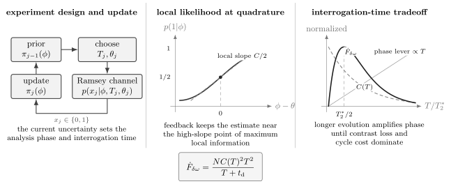
Ramsey sensing is a closed estimation loop. The prior or current estimate sets the interrogation time $T$ and analysis phase $\theta$; the binary outcome updates the likelihood; and the next setting balances local slope, contrast, phase aliases, and wall-clock cost. Increasing $T$ amplifies the phase response but eventually loses information rate through decoherence and dead time.

Periodicity and Dynamic Range

A Ramsey fringe is periodic:

$$p_\theta(1|\phi+2\pi m,C) = p_\theta(1|\phi,C), \qquad m\in\mathbb Z.$$

For fixed $T$, frequency values separated by $2\pi/T$ are aliases. A local uncertainty such as $1/(CT\sqrt{N\nu})$ is meaningful only after the correct fringe branch has been identified. If the prior support is broader than one period, a single interrogation time cannot determine the frequency globally.

Two analysis phases can recover both local quadratures. For example, settings $\theta$ and $\theta+\pi/2$ estimate sine and cosine components, leading to a circular phase estimate

$$\widehat\phi = \theta + \operatorname{atan2} \left( \widehat s, \widehat c \right).$$

Quadrature readout distinguishes phase within a $2\pi$ interval but does not remove the integer alias. Low contrast also makes the angle estimator non-Gaussian; near the origin of the estimated quadrature plane, a symmetric confidence region is usually misleading.

Dynamic range is not just the fringe period. It also depends on prior knowledge, control range, sampling schedule, update latency, drift between settings, and the allowed probability of a cycle slip. A sensitivity number without an unambiguous range or tracking model is incomplete when the signal is not already locked near quadrature.

Multitime and Adaptive Ramsey Estimation

Broad-range protocols combine short and long interrogation times. A short time has weak phase leverage but a wide frequency period; a long time has high local resolution but many aliases. A geometric schedule such as

$$T_k = 2^kT_0$$

can identify coarse frequency bits before refining the estimate. Repetitions at each scale suppress branch errors.

In a Bayesian implementation, the posterior after outcome $x_j$ is

$$\pi_j(\phi) \propto p(x_j|\phi,T_j,\theta_j) \pi_{j-1}(\phi).$$

The next setting may be chosen to minimize expected posterior loss, maximize expected information gain, avoid a cycle slip, or satisfy a latency and bandwidth constraint. Adaptation can change $\theta_j$, $T_j$, or both.

An adaptive protocol must report more than the final posterior width. Its resource ledger includes

• the total phase-accumulation time across all interrogations;
• preparation, readout, reset, and classical computation time;
• the number of probes or channel uses;
• feedback latency and controller bandwidth;
• the prior and the frequency range over which success is evaluated;
• failure tails, branch errors, and stopping rules.

Repeated coherent phase accumulation can exchange spatial entanglement for temporal queries. Such protocols may realize Heisenberg-like query scaling in an ideal phase-estimation problem, but the claim must count every application of the phase and address decoherence and global ambiguity. The canonical resource analysis belongs to Heisenberg Scaling.

Readout Errors and Nuisance Parameters

Let $\alpha$ be the probability of reporting one when the true state is zero, and let $\beta$ be the probability of reporting zero when the true state is one. If the ideal Ramsey probability is $p$, the observed probability is

$$q = \alpha(1-p) + (1-\beta)p.$$

For the sine fringe,

$$q = \frac12 \left[ 1+\alpha-\beta + (1-\alpha-\beta) C\sin(\phi-\theta) \right].$$

Readout asymmetry creates an offset; total classification error reduces the observed contrast. At quadrature the single-outcome Fisher information is

$$F_1 = \frac{ (1-\alpha-\beta)^2C^2 }{ 1-(\alpha-\beta)^2 }.$$

For symmetric error $\alpha=\beta=\epsilon$, this becomes

$$F_1 = (1-2\epsilon)^2C^2.$$

Correcting a fitted contrast by a calibrated readout fidelity can estimate the premeasurement state, but it does not restore information lost by the actual detector. A state-characterization claim and an achieved sensor-sensitivity claim therefore use different noise ledgers.

Contrast $C$, offset $b$, analysis-phase drift, and coupling calibration are often inferred jointly with the signal. For parameters $\boldsymbol\vartheta=(\phi,C,b,\ldots)$, the Fisher matrix is

$$[F(\boldsymbol\vartheta)]_{ab} = \sum_x p(x|\boldsymbol\vartheta) \, \partial_a\ln p \, \partial_b\ln p.$$

If nuisance parameters are unknown, the relevant local bound is

$$\operatorname{Var}(\widehat\phi) \ge [F^{-1}]_{\phi\phi},$$

not $1/F_{\phi\phi}$. Calibration data can add Fisher information, but its shots and elapsed time belong in an end-to-end comparison.

Decoherence and Correlated Noise

The contrast function is an averaged coherence,

$$C(T) = \left| \left\langle e^{i\delta\phi(T)} \right\rangle \right|,$$

where $\delta\phi$ is random phase accumulated from uncontrolled fields or frequency fluctuations. Exponential contrast often indicates approximately Markovian dephasing, while Gaussian decay commonly arises from quasistatic or inhomogeneous detuning. The envelope alone rarely identifies a unique microscopic noise process.

For a stationary classical frequency noise $\delta\omega(t)$, the phase variance can be expressed through a filter function. With

$$Y(\omega) = \int_0^T y(t)e^{i\omega t} \,dt,$$

Gaussian noise gives, up to the convention used for one- or two-sided spectra,

$$C(T) = \exp\left[ -\frac12 \int \frac{d\omega}{2\pi} S_{\delta\omega}(\omega) |Y(\omega)|^2 \right].$$

Ordinary Ramsey evolution has

$$|Y(\omega)|^2 = \frac{ 4\sin^2(\omega T/2) }{ \omega^2 },$$

so it is strongly sensitive to quasistatic and low-frequency detuning. Echo and dynamical-decoupling sequences alter $y(t)$ and shift sensitivity toward selected nonzero frequencies; they answer a different sensing question.

Common-mode phase noise also invalidates naive independent-probe scaling. If all $N$ probes share an unobserved phase $\delta$, then

$$P(K|\phi) = \int d\delta\, P(\delta) \operatorname{Bin} \left[ K;N,p(\phi+\delta) \right].$$

Outcomes are conditionally independent at fixed $\delta$ but correlated after $\delta$ is marginalized. Increasing $N$ can suppress projection noise while leaving a common oscillator or environmental floor unchanged. Likewise, dead-time aliasing can fold oscillator noise into a clock measurement even when each Ramsey shot is otherwise ideal.

Correlated and Entangled Probes

Ramsey interrogation is not restricted to independent qubits. For a collective spin, the first operation prepares a transverse mean spin, the signal rotates it, and the final analysis maps a transverse component to a population difference. A spin-squeezed input can reduce readout noise while retaining signal slope. Its local phase variance is

$$(\Delta\phi)^2 = \frac{\xi_R^2}{N}$$

for an aligned ideal readout. The contrast, squeezed variance, cycle time, and detector noise must all refer to the same operating sequence. Spin Squeezing owns the collective covariance geometry, generation mechanisms, and entanglement criteria.

An ideal $N$-qubit GHZ state,

$$|\mathrm{GHZ}_N\rangle = \frac{ |0\rangle^{\otimes N} + |1\rangle^{\otimes N} }{\sqrt2},$$

accumulates the amplified phase $N\phi$. A parity-like readout can have

$$p(1|\phi) = \frac12 \left[ 1+C_N\sin(N\phi-\theta) \right],$$

and local Fisher information

$$F_\phi = C_N^2N^2$$

at quadrature. The same factor $N$ narrows the unambiguous fringe period to $2\pi/N$, and independent dephasing can make $C_N$ decay rapidly with $N$ and $T$. Under common Markovian dephasing, maximally entangled probes need not improve the asymptotic frequency resolution over optimized uncorrelated Ramsey spectroscopy.

Entanglement can still improve constants, finite-resource performance, or operation under structured noise. The defensible question is not whether the input is entangled, but whether the complete protocol improves the declared loss under the same time, probe, prior, bandwidth, and success conditions.

Representative Sensing Mappings

The Ramsey information structure is portable, but each platform supplies a different phase response and noise model.

Task	Encoded phase	Essential calibration	Common limiting noise
Frequency comparison	$\phi=(\omega_0-\omega_{\mathrm{LO}})T$	interrogation time and oscillator phase	local-oscillator noise, dead time, collisions
DC magnetometry	$\phi=\gamma BT$	gyromagnetic ratio and field projection	$T_2^*$ dephasing, field drift, readout noise
Electric-field sensing	$\phi=\int\Delta\omega_E(t)dt$	Stark response and field geometry	electric-field noise, level mixing, calibration drift
Inertial phase readout	platform-dependent action phase	scale factor, timing, trajectory	vibration, laser phase, wave-front error
Qubit calibration	$\phi=\delta\omega T+\phi_c$	pulse phase and timing	control drift, leakage, correlated phase noise

For a spin with Hamiltonian

$$H_B = \frac{\hbar\gamma B}{2} \sigma_z,$$

the phase is $\phi=\gamma BT$. The projection-noise-limited field sensitivity per square root bandwidth is

$$\eta_B \ge \frac{ \sqrt{T_c} }{ \gamma C(T)T\sqrt N }.$$

This formula is useful only after specifying whether $N$ counts simultaneous probes, repeated probes, detected probes, or accepted probes. Spatial resolution, standoff distance, sensor volume, and invasiveness can be as important as field sensitivity in an application.

An End-to-End Analysis Workflow

A reliable Ramsey analysis can be organized as the following sequence.

1. Declare the estimand. State whether the target is phase, frequency, field amplitude, a time-dependent waveform coefficient, or a decision.
2. Specify the response. Give $\phi(\lambda,T)$, its units, sign convention, and calibration uncertainty.
3. Write the outcome model. Include contrast, offset, readout confusion, atom-number variation, and any shared latent phase.
4. State the operating policy. Report $T$, $\theta$, adaptation, phase steps, stopping rule, and allowed prior range.
5. Fit or update the full likelihood. Preserve periodicity until a phase branch is justified.
6. Validate uncertainty. Use repeated data, simulation, posterior calibration, or confidence-interval coverage tests under the stated noise model.
7. Convert to wall-clock performance. Include preparation, control, readout, reset, feedback, discarded trials, and downtime.
8. Audit the comparator. Match probe exposure, elapsed time, bandwidth, prior information, calibration data, and success criterion.

Residual plots and fitted contrast are not enough when temporal correlation is plausible. Inspect block averages, autocorrelation, Allan-type statistics, or a state-space model appropriate to the application. A likelihood that treats drift as independent shot noise can produce uncertainty intervals that are precise and wrong.

What Different Results Establish

Reported result	What it supports	What it does not establish alone
A high-contrast fringe	coherent preparation, phase accumulation, and recombination	calibrated sensitivity or sensor advantage
A measured $T_2^*$	an operational Ramsey coherence envelope	a unique microscopic noise spectrum
Projection-noise scaling with $N$	consistency with independent population statistics over the tested range	absence of common-mode floors at larger $N$
Local Fisher information	information near a stated working point under a likelihood	global identifiability or unbiased finite-data performance
QFI of the prepared state	a measurement-optimized local bound under the state model	attainment by the implemented detector
Sensitivity in units per $\sqrt{\mathrm{Hz}}$	time-normalized precision under a stated duty cycle	accuracy, bandwidth, spatial resolution, or long-term stability
Spin-squeezed Ramsey gain	reduced phase variance for a matched local readout	complete clock improvement unless cycle and oscillator noise are included
An adaptive posterior	inference conditioned on the prior and model	calibrated coverage under drift or model misspecification

A strong Ramsey claim therefore gives both the number and the contract around the number. The contract should identify the dataset boundary, nuisance model, calibration provenance, estimator, uncertainty method, resource ledger, and failure probability.

Common Mistakes

• Calling a visible fringe a precision measurement without defining an estimator or uncertainty.
• Operating near a fringe maximum while applying linear error propagation as if the slope were maximal.
• Quoting $1/(CT\sqrt N)$ without cycle time, repetitions, or units.
• Treating $T_2^*$ as an interrogation time that is automatically optimal for every objective.
• Ignoring the $2\pi$ phase ambiguity when the prior spans several fringes.
• Subtracting detector noise to claim an achieved sensitivity without also reporting the raw detector-level result.
• Inverting $F_{\phi\phi}$ while jointly fitted nuisance parameters are correlated with phase.
• Assuming atom outcomes are independent after averaging over common oscillator or environmental noise.
• Equating QFI with the Fisher information of the implemented readout.
• Claiming Heisenberg scaling from a narrower $N\phi$ fringe without counting branch resolution, coherence loss, and every phase query.
• Comparing an entangled protocol with an unsqueezed baseline that has a different duty cycle, prior, loss, or accepted-shot rule.
• Interpreting a coherence envelope as a unique noise spectrum without an identified filter-function model.

Exercises

1. Fisher information of a contrast-reduced fringe

For

$$p(1|\phi) = \frac12 \left(1+C\sin\phi\right),$$

derive the one-shot Fisher information and evaluate it at $\phi=0$.

Solution

The derivative is

$$\partial_\phi p = \frac{C}{2}\cos\phi.$$

For a Bernoulli outcome,

$$F_1 = \frac{(\partial_\phi p)^2}{p(1-p)}.$$

Since

$$p(1-p) = \frac14 \left(1-C^2\sin^2\phi\right),$$

we obtain

$$F_1(\phi) = \frac{ C^2\cos^2\phi }{ 1-C^2\sin^2\phi }.$$

At quadrature, $\phi=0$, so $F_1=C^2$.

2. Projection-noise estimator

$N$ independent probes are operated at quadrature with known contrast $C$. Let $f=K/N$. Show that

$$\widehat\phi = \frac{2f-1}{C}$$

is locally unbiased at $\phi=0$ and find its variance there.

Solution

Near zero,

$$\mathbb E[f] = \frac12(1+C\sin\phi) \simeq \frac12(1+C\phi).$$

Therefore

$$\mathbb E[\widehat\phi] \simeq \phi.$$

At $\phi=0$, $p=1/2$ and

$$\operatorname{Var}(f) = \frac{p(1-p)}{N} = \frac{1}{4N}.$$

Thus

$$\operatorname{Var}(\widehat\phi) = \frac{4}{C^2} \operatorname{Var}(f) = \frac{1}{NC^2}.$$

3. Optimal time under exponential dephasing

Assume negligible dead time and

$$C(T)=e^{-T/T_2^*}.$$

Find the interrogation time that maximizes frequency Fisher information per unit time.

Solution

The information per cycle is proportional to $C(T)^2T^2$. With cycle time $T$, the information rate is proportional to

$$R(T) = Te^{-2T/T_2^*}.$$

Its logarithmic derivative is

$$\frac{d}{dT}\ln R = \frac1T - \frac{2}{T_2^*}.$$

The maximum occurs at

$$T_{\mathrm{opt}} = \frac{T_2^*}{2}.$$

Maximizing single-shot information instead would give $T=T_2^*$, showing why the time objective must be stated.

4. Readout confusion

Take symmetric state-classification error $\alpha=\beta=\epsilon=0.05$ and intrinsic contrast $C=0.8$. Find the observed contrast and one-outcome Fisher information at quadrature.

Solution

Symmetric confusion multiplies contrast by $1-2\epsilon$, so

$$C_{\mathrm{obs}} = (1-2\epsilon)C = 0.9\times0.8 = 0.72.$$

At quadrature,

$$F_1 = C_{\mathrm{obs}}^2 = 0.5184.$$

Correcting the contrast can infer the state before readout, but the detector still extracts only this smaller amount of information per outcome.

5. Frequency aliases

A Ramsey experiment uses $T=20\,\mathrm{ms}$. By how much can angular frequency change while producing the same ideal fringe? Give the corresponding ordinary-frequency spacing.

Solution

The fringe is unchanged when

$$\delta\omega T \longrightarrow \delta\omega T+2\pi m.$$

Adjacent angular-frequency aliases are separated by

$$\Delta\omega_{\mathrm{alias}} = \frac{2\pi}{T} = 100\pi\,\mathrm{rad\,s^{-1}}.$$

The ordinary-frequency spacing is

$$\Delta f_{\mathrm{alias}} = \frac{1}{T} = 50\,\mathrm{Hz}.$$

6. Duty-cycle penalty

Two protocols have the same $N$, contrast, and interrogation time $T$. Protocol A has no dead time, while protocol B has $t_{\mathrm d}=3T$. Compare their frequency standard deviations after the same wall-clock averaging time.

Solution

The variance scales with cycle time $T_c=T+t_{\mathrm d}$. Hence

$$\frac{ \Delta\widehat{\delta\omega}_B }{ \Delta\widehat{\delta\omega}_A } = \sqrt{ \frac{T_{c,B}}{T_{c,A}} } = \sqrt{ \frac{4T}{T} } = 2.$$

Protocol B has twice the standard deviation after equal wall-clock time, despite identical one-shot statistics.

7. GHZ resolution and range

Compare an ideal $N$-qubit GHZ Ramsey fringe with an independent-probe fringe. What happens to local Fisher information and unambiguous phase period?

Solution

At quadrature and unit contrast, the GHZ fringe depends on $N\phi$, so

$$F_{\phi,\mathrm{GHZ}} = N^2.$$

$N$ independent probes give total information $N$. The GHZ state therefore has an ideal factor-$N$ local information gain for the same simultaneous probe count. Its fringe period is

$$\frac{2\pi}{N},$$

instead of $2\pi$. The local gain is accompanied by a factor-$N$ reduction in unambiguous phase range, before including GHZ preparation cost or faster decoherence.

8. A magnetic-field sensitivity

An ensemble of $N=10^4$ independent spins has $\gamma=2\pi\times28\,\mathrm{GHz\,T^{-1}}$, $T=1\,\mu\mathrm{s}$, $C=0.7$, and $T_c=5\,\mu\mathrm{s}$. Estimate the projection-noise-limited $\eta_B$.

Solution

Use

$$\eta_B = \frac{\sqrt{T_c}}{\gamma CT\sqrt N}.$$

Substitution gives

$$\begin{aligned} \eta_B &= \frac{ \sqrt{5\times10^{-6}\,\mathrm s} }{ (2\pi)(28\times10^9\,\mathrm{s^{-1}T^{-1}}) (0.7)(10^{-6}\,\mathrm s)(100) } \\ &\simeq 1.8\times10^{-10} \,\mathrm{T\,Hz^{-1/2}}. \end{aligned}$$

This is about $180\,\mathrm{pT\,Hz^{-1/2}}$. It is a model benchmark, not a complete instrument sensitivity: calibration noise, spatial response, technical phase noise, and long-term drift are absent.

References

1. N. F. Ramsey, “A molecular beam resonance method with separated oscillating fields,” Physical Review 78, 695–699 (1950), doi:10.1103/PhysRev.78.695.
2. W. M. Itano, J. C. Bergquist, J. J. Bollinger, J. M. Gilligan, D. J. Heinzen, F. L. Moore, M. G. Raizen, and D. J. Wineland, “Quantum projection noise: Population fluctuations in two-level systems,” Physical Review A 47, 3554–3570 (1993), doi:10.1103/PhysRevA.47.3554.
3. D. J. Wineland, J. J. Bollinger, W. M. Itano, and D. J. Heinzen, “Squeezed atomic states and projection noise in spectroscopy,” Physical Review A 50, 67–88 (1994), doi:10.1103/PhysRevA.50.67.
4. S. L. Braunstein and C. M. Caves, “Statistical distance and the geometry of quantum states,” Physical Review Letters 72, 3439–3443 (1994), doi:10.1103/PhysRevLett.72.3439.
5. S. F. Huelga, C. Macchiavello, T. Pellizzari, A. K. Ekert, M. B. Plenio, and J. I. Cirac, “Improvement of frequency standards with quantum entanglement,” Physical Review Letters 79, 3865–3868 (1997), doi:10.1103/PhysRevLett.79.3865.
6. G. Santarelli, Ph. Laurent, P. Lemonde, A. Clairon, A. G. Mann, S. Chang, A. N. Luiten, and C. Salomon, “Quantum projection noise in an atomic fountain: A high stability cesium frequency standard,” Physical Review Letters 82, 4619–4622 (1999), doi:10.1103/PhysRevLett.82.4619.
7. M. G. A. Paris, “Quantum estimation for quantum technology,” International Journal of Quantum Information 7, 125–137 (2009), doi:10.1142/S0219749909004839.
8. B. M. Escher, R. L. de Matos Filho, and L. Davidovich, “General framework for estimating the ultimate precision limit in noisy quantum-enhanced metrology,” Nature Physics 7, 406–411 (2011), doi:10.1038/nphys1958.
9. R. Demkowicz-Dobrzański, J. Kołodyński, and M. Guță, “The elusive Heisenberg limit in quantum-enhanced metrology,” Nature Communications 3, 1063 (2012), doi:10.1038/ncomms2067.
10. G. Tóth and I. Apellaniz, “Quantum metrology from a quantum information science perspective,” Journal of Physics A 47, 424006 (2014), doi:10.1088/1751-8113/47/42/424006.
11. L. Pezzè, A. Smerzi, M. K. Oberthaler, R. Schmied, and P. Treutlein, “Quantum metrology with nonclassical states of atomic ensembles,” Reviews of Modern Physics 90, 035005 (2018), doi:10.1103/RevModPhys.90.035005.
12. C. L. Degen, F. Reinhard, and P. Cappellaro, “Quantum sensing,” Reviews of Modern Physics 89, 035002 (2017), doi:10.1103/RevModPhys.89.035002.
13. Ł. Cywiński, R. M. Lutchyn, C. P. Nave, and S. Das Sarma, “How to enhance dephasing time in superconducting qubits,” Physical Review B 77, 174509 (2008), doi:10.1103/PhysRevB.77.174509.
14. D. W. Berry and H. M. Wiseman, “Optimal states and almost optimal adaptive measurements for quantum interferometry,” Physical Review Letters 85, 5098–5101 (2000), doi:10.1103/PhysRevLett.85.5098.
15. B. L. Higgins, D. W. Berry, S. D. Bartlett, H. M. Wiseman, and G. J. Pryde, “Entanglement-free Heisenberg-limited phase estimation,” Nature 450, 393–396 (2007), doi:10.1038/nature06257.
16. A. Said, D. W. Berry, and J. Twamley, “Nanoscale magnetometry using a single-spin system in diamond,” Physical Review B 83, 125410 (2011), doi:10.1103/PhysRevB.83.125410.
17. C. Bonato et al., “Optimized quantum sensing with a single electron spin using real-time adaptive measurements,” Nature Nanotechnology 11, 247–252 (2016), doi:10.1038/nnano.2015.261.
18. E. M. Kessler, P. Kómár, M. Bishof, L. Jiang, A. S. Sørensen, J. Ye, and M. D. Lukin, “Heisenberg-limited atom clocks based on entangled qubits,” Physical Review Letters 112, 190403 (2014), doi:10.1103/PhysRevLett.112.190403.
19. M. Schulte, C. Lisdat, P. O. Schmidt, U. Sterr, and K. Hammerer, “Prospects and challenges for squeezing-enhanced optical atomic clocks,” Nature Communications 11, 5955 (2020), doi:10.1038/s41467-020-19403-7.
20. C. W. Chou, D. B. Hume, M. J. Thorpe, D. J. Wineland, and T. Rosenband, “Quantum coherence between two atoms beyond $Q=10^{15}$,” Physical Review Letters 106, 160801 (2011), doi:10.1103/PhysRevLett.106.160801.
21. E. Oelker et al., “Demonstration of $4.8\times10^{-17}$ stability at 1 s for two independent optical clocks,” Nature Photonics 13, 714–719 (2019), doi:10.1038/s41566-019-0493-4.
22. M. Schioppo et al., “Ultrastable optical clock with two cold-atom ensembles,” Nature Photonics 11, 48–52 (2017), doi:10.1038/nphoton.2016.231.

Further Connections

• Ramsey Interferometry derives the pulse sequence, finite-pulse line shape, fringe width, spectroscopy conventions, and experimental diagnostics.
• Quantum Measurement as Estimation supplies the estimand, likelihood, estimator, loss, uncertainty, and validation contract used here.
• Classical and Quantum Fisher Information develops the measurement-dependent information, SLD metric, and attainability caveats behind the Ramsey bounds.
• Cramér–Rao Bounds explains regularity, bias, nuisance parameters, finite samples, and global alternatives.
• Standard Quantum Limit owns the independent-probe benchmark and matched-resource comparison.
• Heisenberg Scaling treats sequential queries, entangled probes, phase ambiguity, nonlinear generators, and noisy asymptotes.
• Spin Squeezing develops collective-spin covariance, Wineland gain, entanglement certification, and squeezing-enhanced Ramsey readout.
• Mach–Zehnder Interferometry translates the same prepare–encode–measure logic to optical paths while making phase references, photon loss, multipass queries, and sample dose explicit.
• Atomic Clocks closes repeated Ramsey interrogations around a noisy oscillator and develops state-space tracking, phase-slip reliability, and clock-level quantum-gain claims.
• Noise and Decoherence in Metrology compares product and GHZ Ramsey probes after coherence loss, dead time, channel bounds, correlated noise, and control are included.
• Rabi and Ramsey Control compares free-induction, echo, and driven-control protocols in open systems.
• Noise Spectra owns spectral conventions and the connection between temporal correlations and filter functions.
• Sensing Case Studies audits clocks, magnetometers, atom interferometers, and electrometers under end-to-end evidence standards.