Classical and Quantum Fisher Information

Fisher information quantifies how quickly nearby parameter values become statistically distinguishable. In a quantum experiment there are two distinct levels:

• classical Fisher information $F_C$ belongs to the outcome distribution produced by a specified measurement;
• quantum Fisher information $F_Q$ is the greatest classical Fisher information available from the parameterized quantum state when all allowed measurements are considered.

That distinction is operational. A state may contain information that the implemented detector does not extract. Conversely, a reported $F_Q$ does not identify a realizable detector, remove nuisance parameters, resolve global aliases, or guarantee good finite-sample performance.

This page is the canonical home for measurement-induced Fisher information, the symmetric logarithmic derivative (SLD), spectral and pure-state formulas, the Braunstein–Caves measurement optimization, quantum information geometry, and multiparameter compatibility. Fisher Information owns the classical score, regularity assumptions, and generic statistical derivations. Quantum Measurement as Estimation owns the full experimental contract from estimand to validated report. Standard Quantum Limit owns independent-probe scaling and matched-resource comparisons.

The Statistical Model Comes First

Let a real parameter $\theta$ be encoded in a density operator $\rho_\theta$. A parameter-independent POVM

$$\mathsf M=\{M_x\}_x, \qquad M_x\succeq0, \qquad \sum_x M_x=I,$$

produces the probabilities

$$p(x\mid\theta,\mathsf M) = \operatorname{Tr}(\rho_\theta M_x).$$

For discrete outcomes, the classical Fisher information of this measurement is

$$F_C(\theta;\mathsf M) = \sum_{x:p_x>0} \frac{(\partial_\theta p_x)^2}{p_x}, \qquad p_x=\operatorname{Tr}(\rho_\theta M_x).$$

For a continuous record, replace the sum by an integral with respect to the declared reference measure. Outcomes whose probability vanishes require a limit or a support-sensitive treatment; silently inserting $p_x=0$ into the fraction is not meaningful.

The notation $F_C(\theta;\mathsf M)$ deliberately names the measurement. Changing the basis, detector resolution, acceptance rule, or coarse graining changes the likelihood and can change the available information.

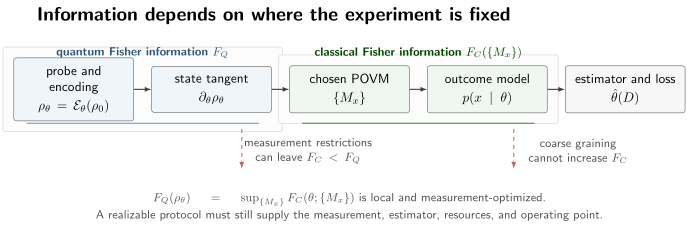
Quantum Fisher information belongs to the local state tangent before a measurement is fixed. Classical Fisher information belongs to the likelihood afterward. Measurement restrictions and classical coarse graining can discard information; an estimator and resource model are still needed to turn either quantity into a precision claim.

Classical Fisher Information After Measurement

The score of one observed outcome is

$$s_\theta(x) = \partial_\theta\log p(x\mid\theta,\mathsf M).$$

Under the usual regularity assumptions, $\mathbb E_\theta[s_\theta]=0$, and

$$F_C(\theta;\mathsf M) = \mathbb E_\theta[s_\theta^2].$$

Thus $F_C$ is a local signal-to-noise ratio for the score. If $\theta$ changes the probabilities strongly compared with their statistical fluctuations, $F_C$ is large. If all probabilities are locally stationary, $F_C=0$ for that measurement even when another measurement would be informative.

For $\nu$ independent repetitions of the same measurement,

$$F_C^{(\nu)} = \nu F_C^{(1)}.$$

This additivity is a statement about independent likelihoods, not about every experiment containing $\nu$ nominal shots. Drift, temporal correlations, adaptive settings, dead time, and postselection must be represented in the actual joint likelihood.

Classical postprocessing cannot increase Fisher information. If $y$ is generated from $x$ by a parameter-independent stochastic map $K(y\mid x)$, then

$$F_C(Y;\theta) \le F_C(X;\theta).$$

Discarding time tags, binning a continuous signal too coarsely, thresholding an analog record, or merging detector outcomes may therefore lose sensitivity.

Quantum Fisher Information as an Optimization

For a one-parameter state family, the SLD quantum Fisher information is

$$F_Q(\theta) = \sup_{\mathsf M} F_C(\theta;\mathsf M),$$

where the supremum is over parameter-independent POVMs on the system at the specified operating point. In a regular finite-dimensional one-parameter model, this supremum is attained locally by a projective measurement in an eigenbasis of the SLD defined below.

The optimization has three important qualifications:

1. It is local in $\theta$. It compares infinitesimally neighboring states, not all parameter values across a wide prior interval.
2. The optimizing measurement can depend on the unknown true value. Practical protocols use prior localization, adaptive measurements, covariant constructions, or a detector that is near-optimal over a declared range.
3. The optimization must respect the physical measurement class. If only a restricted set $\mathcal A$ is implementable, the relevant quantity is

$$F_{\mathcal A}(\theta) = \sup_{\mathsf M\in\mathcal A} F_C(\theta;\mathsf M),$$

which may be strictly smaller than $F_Q$.

Symmetric Logarithmic Derivative

The symmetric logarithmic derivative $L_\theta$ is a Hermitian operator satisfying

$$\partial_\theta\rho_\theta = \frac12 \left( L_\theta\rho_\theta + \rho_\theta L_\theta \right).$$

The corresponding quantum Fisher information is

$$\begin{aligned} F_Q(\theta) &= \operatorname{Tr}(\rho_\theta L_\theta^2)\\ &= \operatorname{Tr} \left[ (\partial_\theta\rho_\theta)L_\theta \right]. \end{aligned}$$

If $\rho_\theta$ is not full rank, $L_\theta$ need not be unique on the kernel of $\rho_\theta$. Its action on the support determines $F_Q$, so this nonuniqueness does not change the value in a regular fixed-rank model. Points where rank or support changes deserve separate care: the SLD expression, its nearby limit, and finite-difference distinguishability need not behave as a naive smooth formula suggests.

The SLD is not usually an observable that the parameter encoding literally couples to. It is the locally optimal score operator for the quantum model.

Why Every Measurement Obeys the Quantum Bound

For a fixed POVM element $M_x$,

$$\begin{aligned} \partial_\theta p_x &= \operatorname{Tr} \left[ (\partial_\theta\rho_\theta)M_x \right]\\ &= \operatorname{Re} \operatorname{Tr} (\rho_\theta L_\theta M_x). \end{aligned}$$

A Hilbert–Schmidt Cauchy–Schwarz inequality gives

$$(\partial_\theta p_x)^2 \le p_x\, \operatorname{Tr} (\rho_\theta L_\theta M_x L_\theta).$$

Summing over outcomes yields the Braunstein–Caves inequality,

$$\begin{aligned} F_C(\theta;\mathsf M) &\le \sum_x \operatorname{Tr} (\rho_\theta L_\theta M_x L_\theta)\\ &= \operatorname{Tr}(\rho_\theta L_\theta^2)\\ &= F_Q(\theta). \end{aligned}$$

At a known operating point, measuring the spectral projectors of $L_\theta$ saturates the scalar bound under the regularity conditions. This proves a local optimization statement. It does not prove that one fixed detector is globally optimal or that the resulting estimator reaches a variance bound for a finite data set.

Spectral Formula for Mixed States

Write the spectral decomposition

$$\rho_\theta = \sum_i \lambda_i \lvert i\rangle\langle i\rvert.$$

In this instantaneous eigenbasis, the SLD matrix elements on the support are

$$\langle i|L_\theta|j\rangle = \frac{ 2\langle i|\partial_\theta\rho_\theta|j\rangle }{ \lambda_i+\lambda_j }, \qquad \lambda_i+\lambda_j>0.$$

Therefore

$$F_Q(\theta) = 2 \sum_{i,j:\lambda_i+\lambda_j>0} \frac{ |\langle i|\partial_\theta\rho_\theta|j\rangle|^2 }{ \lambda_i+\lambda_j }.$$

Separating eigenvalue and eigenvector changes gives

$$\begin{aligned} F_Q ={}& \sum_{i:\lambda_i>0} \frac{(\partial_\theta\lambda_i)^2}{\lambda_i}\\ &+ 2\sum_{i\ne j:\lambda_i+\lambda_j>0} \frac{(\lambda_i-\lambda_j)^2}{\lambda_i+\lambda_j} |\langle i|\partial_\theta j\rangle|^2. \end{aligned}$$

The first line is information in changing eigenvalues and is classical in the instantaneous eigenbasis. The second is information in rotating eigenvectors, which requires a measurement sensitive to coherence between those directions.

For a commuting family,

$$[\rho_\theta,\rho_{\theta'}]=0 \quad \text{for all nearby }\theta,\theta',$$

one common eigenbasis measures all the available information, and $F_Q$ reduces to the classical Fisher information of the eigenvalues.

Pure-State Formula

For a differentiable normalized state $\lvert\psi_\theta\rangle$, write

$$\lvert\dot\psi_\theta\rangle = \partial_\theta\lvert\psi_\theta\rangle.$$

The pure-state quantum Fisher information is

$$F_Q[\lvert\psi_\theta\rangle] = 4 \left( \langle\dot\psi_\theta|\dot\psi_\theta\rangle - |\langle\psi_\theta|\dot\psi_\theta\rangle|^2 \right).$$

The subtraction removes parameter-dependent global phase. If $\lvert\psi_\theta\rangle=e^{i\chi(\theta)}\lvert\psi_0\rangle$, the ray does not change and $F_Q=0$.

For a unitary encoding

$$\lvert\psi_\theta\rangle = e^{-i\theta G} \lvert\psi_0\rangle,$$

with a parameter-independent Hermitian generator $G$,

$$F_Q = 4\operatorname{Var}_{\psi_0}(G).$$

This identity is exact for pure states. For a mixed input under the same unitary encoding,

$$F_Q[\rho,G] = 2 \sum_{i,j:\lambda_i+\lambda_j>0} \frac{(\lambda_i-\lambda_j)^2}{\lambda_i+\lambda_j} |\langle i|G|j\rangle|^2,$$

and only the inequality

$$F_Q[\rho,G] \le 4\operatorname{Var}_\rho(G)$$

holds in general. A mixed state can have nonzero generator variance entirely from classical uncertainty while commuting with $G$; then the state does not move under the encoding and its QFI is zero.

Example: A Qubit Phase

Consider

$$\lvert\psi_\theta\rangle = \frac{ \lvert0\rangle+e^{i\theta}\lvert1\rangle }{\sqrt2}.$$

Direct substitution into the pure-state formula gives

$$F_Q=1.$$

At a provisional operating point $\theta_0$, measure the observable

$$Y_{\theta_0} = -\sin\theta_0\,X + \cos\theta_0\,Y.$$

Its two outcome probabilities are

$$p_\pm(\theta) = \frac12 \left[ 1\pm\sin(\theta-\theta_0) \right].$$

At $\theta=\theta_0$,

$$F_C(\theta_0;Y_{\theta_0}) = 1 = F_Q.$$

The detector is locally optimal because it measures the quadrature with the largest slope at the operating point. But the state and likelihood are periodic, so $F_Q=1$ alone cannot identify which $2\pi$ branch contains the true phase. Dynamic range and phase unwrapping belong to the full estimation protocol.

Example: A Commuting Qubit Family

Let

$$\rho_\theta = \theta\lvert0\rangle\langle0\rvert + (1-\theta)\lvert1\rangle\langle1\rvert, \qquad 0<\theta<1.$$

Only the eigenvalues change. Measuring in the computational basis gives a Bernoulli model and

$$F_C = \frac1\theta+ \frac1{1-\theta} = \frac1{\theta(1-\theta)}.$$

The spectral QFI formula gives the same result, so

$$F_Q = F_C(Z).$$

No coherent measurement is needed because the model is already classical in a common basis. The divergence near $\theta=0$ or $1$ is also a warning: boundary points violate some regularity assumptions behind familiar local asymptotic conclusions.

Example: Dephased Phase Sensing

An equatorial qubit with reduced coherence can be written

$$\rho_\theta = \frac12 \left[ I+ \eta (\cos\theta\,X+\sin\theta\,Y) \right], \qquad 0\le\eta\le1.$$

Its Bloch vector has constant length $\eta$ and rotates in the equatorial plane. The qubit formula derived below gives

$$F_Q(\theta)=\eta^2.$$

If the unknown parameter is a frequency $\omega$, the phase is $\theta=\omega t$, and Markovian dephasing gives $\eta=e^{-\gamma t}$, then one interrogation has

$$F_Q^{(1)}(\omega;t) = t^2e^{-2\gamma t}.$$

Ignoring dead time, a total duration $T$ permits about $T/t$ independent interrogations, so

$$F_Q^{\rm tot} = Tt\,e^{-2\gamma t}.$$

This is maximized at $t=1/(2\gamma)$. Longer coherent evolution increases the phase slope but also destroys contrast. The useful optimization variable is therefore not state QFI in isolation, but total information under the declared time and noise model.

Bloch-Vector Formula

For a full-rank qubit

$$\rho_\theta = \frac12 \left(I+\mathbf r_\theta\boldsymbol\cdot\boldsymbol\sigma\right), \qquad |\mathbf r_\theta|<1,$$

the QFI is

$$F_Q = |\partial_\theta\mathbf r|^2 + \frac{ (\mathbf r\boldsymbol\cdot\partial_\theta\mathbf r)^2 }{ 1-|\mathbf r|^2 }.$$

The first term measures motion of the Bloch vector. The second records changes in its length, weighted more strongly near the pure-state boundary. For a smooth path that stays pure, $|\mathbf r|=1$ and $\mathbf r\boldsymbol\cdot\partial_\theta\mathbf r=0$; taking the appropriate tangent limit gives

$$F_Q=|\partial_\theta\mathbf r|^2.$$

One should not substitute $|\mathbf r|=1$ directly into the full-rank formula. The apparent $0/0$ is the coordinate trace of a rank boundary.

Geometry of Neighboring States

Define the squared Uhlmann fidelity by

$$\mathcal F(\rho,\sigma) = \left[ \operatorname{Tr} \sqrt{\sqrt\rho\,\sigma\sqrt\rho} \right]^2$$

and the Bures distance by

$$D_B^2(\rho,\sigma) = 2\left(1-\sqrt{\mathcal F(\rho,\sigma)}\right).$$

With these conventions, neighboring states obey

$$D_B^2 (\rho_\theta,\rho_{\theta+d\theta}) = \frac14F_Q(\theta)d\theta^2 + o(d\theta^2).$$

Thus QFI is four times the Bures metric evaluated on the parameter tangent. It quantifies local state-space distinguishability before a detector is chosen.

For pure states, the Bures metric reduces locally to the Fubini–Study metric:

$$ds_{\rm FS}^2 = \left( \langle\dot\psi|\dot\psi\rangle - |\langle\psi|\dot\psi\rangle|^2 \right)d\theta^2 = \frac14F_Qd\theta^2.$$

Fubini–Study Geometry owns the projective geometry and convention choices. Here the same line element is interpreted as metrological sensitivity along a specified family.

Structural Properties

Several properties make SLD QFI useful for auditing sensing protocols.

Reparameterization

If $\phi=g(\theta)$ is smooth and locally invertible, then

$$F_Q^{(\phi)} = F_Q^{(\theta)} \left( \frac{d\theta}{d\phi} \right)^2.$$

QFI has units inverse to the square of the parameter. A numerical value is not meaningful until the parameter coordinate and units are named.

Additivity

For independently prepared state families,

$$F_Q(\rho_\theta\otimes\sigma_\theta) = F_Q(\rho_\theta)+F_Q(\sigma_\theta).$$

Hence $N$ independent identical probes carry $NF_Q^{(1)}$. This is the information-theoretic origin of the inverse-square-root precision scaling developed on the Standard Quantum Limit page.

Convexity

For parameter-independent mixing probabilities $q_k$,

$$F_Q \left( \sum_k q_k\rho_{k,\theta} \right) \le \sum_k q_kF_Q(\rho_{k,\theta}).$$

Unrecorded classical mixing cannot improve sensitivity. If the weights $q_k(\theta)$ themselves depend on the parameter, they carry classical information and the useful extended bound is

$$F_Q \left( \sum_k q_k(\theta)\rho_{k,\theta} \right) \le F_C(\{q_k\}) + \sum_k q_kF_Q(\rho_{k,\theta}).$$

Data Processing

For a parameter-independent quantum channel $\Lambda$,

$$F_Q[\Lambda(\rho_\theta)] \le F_Q(\rho_\theta).$$

Measurement is such a channel from a quantum state to a classical register, so this monotonicity contains $F_C\le F_Q$ as a special case. Noise after encoding cannot create information about $\theta$ if the noise mechanism itself has no parameter dependence.

If a device or measurement depends on $\theta$, its dependence can add a new encoding pathway. It must be included in the physical model; it is not a counterexample to parameter-independent data processing.

Recorded Classical Flags

Suppose orthogonal flag states preserve which branch occurred:

$$\rho_\theta^{XQ} = \sum_k q_k(\theta) \lvert k\rangle\langle k\rvert \otimes \rho_{k,\theta}.$$

Then the information decomposes exactly as

$$F_Q(\rho_\theta^{XQ}) = F_C(\{q_k\}) + \sum_k q_kF_Q(\rho_{k,\theta}).$$

This formula is useful for heralding, erasure flags, and branch-resolved experiments. Throwing away the flag applies a channel and can only reduce the information.

From Information to a Variance Bound

For a locally unbiased scalar estimator based on $\nu$ independent copies, the classical and quantum Cramér–Rao inequalities form the chain

$$\operatorname{Var}_\theta(\hat\theta) \ge \frac{1}{\nu F_C(\theta;\mathsf M)} \ge \frac{1}{\nu F_Q(\theta)}.$$

Each inequality has its own attainability question. The first depends on the estimator, sample size, model regularity, and likelihood. The second depends on the measurement and operating point. Equality in both generally requires a measurement that extracts the QFI and an estimator operating in a regime where the classical bound is attainable.

Cramér–Rao Bounds owns the full hierarchy of local-unbiased, biased, Bayesian, finite-sample, and multiparameter bounds. The formula here is a bridge: it explains why $F_Q$ is a precision benchmark, not an achieved error bar.

Multiparameter Quantum Fisher Matrix

For parameters $\boldsymbol\theta=(\theta^1,\ldots,\theta^m)$, define one SLD for each tangent direction,

$$\partial_\mu\rho = \frac12 (L_\mu\rho+\rho L_\mu).$$

The SLD quantum Fisher information matrix is

$$\begin{aligned} (J_Q)_{\mu\nu} &= \frac12 \operatorname{Tr} \left[ \rho\{L_\mu,L_\nu\} \right]\\ &= \operatorname{Re} \operatorname{Tr}(\rho L_\mu L_\nu). \end{aligned}$$

For any real direction $\mathbf u$ in parameter space,

$$\mathbf u^{\mathsf T}J_Q\mathbf u$$

is the scalar QFI for motion along that direction. A singular $J_Q$ indicates at least one locally unidentifiable combination of parameters.

The formal SLD matrix bound is

$$\operatorname{Cov}(\hat{\boldsymbol\theta}) \succeq \frac1\nu J_Q^{-1},$$

under local-unbiasedness and regularity assumptions. Unlike the scalar case, one measurement need not attain all matrix directions simultaneously. The SLDs can encode incompatible optimal observables.

If the SLDs commute on the support of $\rho$, a common eigenbasis removes this obstruction. A weaker mean-commutator condition,

$$\operatorname{Tr} \left[ \rho[L_\mu,L_\nu] \right] =0,$$

is the relevant compatibility criterion for asymptotic saturation in broad regular models with collective measurements. When incompatibility remains, weighted scalar costs and the Holevo Cramér–Rao bound give the operational joint limit; optimizing each diagonal element of $J_Q$ separately overstates what one common experiment can deliver.

Nuisance Parameters

Partition the parameter vector into a target $\alpha$ and nuisance parameters $\boldsymbol\lambda$. Formally partition the QFI matrix as

$$J_Q = \begin{pmatrix} J_{\alpha\alpha} & J_{\alpha\lambda}\\ J_{\lambda\alpha} & J_{\lambda\lambda} \end{pmatrix}.$$

When the relevant inverses and attainability assumptions hold, the Schur complement

$$J_{\rm eff} = J_{\alpha\alpha} - J_{\alpha\lambda} J_{\lambda\lambda}^{-1} J_{\lambda\alpha}$$

is the information remaining about $\alpha$ when $\boldsymbol\lambda$ must also be inferred. It is no larger than $J_{\alpha\alpha}$. Calibration drift, unknown contrast, loss, phase offsets, and background rates can therefore erase an apparent one-parameter advantage.

For a quantum model this Schur complement is an SLD-based local benchmark. It does not remove multiparameter measurement incompatibility; a complete claim must analyze the attainable cost for the joint model.

Channel Quantum Fisher Information

Often the unknown parameter belongs to a channel $\mathcal E_\theta$, not to a state supplied in advance. A single-use, ancilla-assisted channel QFI can be defined by

$$\mathcal F_Q(\mathcal E_\theta) = \sup_{\rho_{SA}} F_Q \left[ (\mathcal E_\theta\otimes\mathcal I_A)(\rho_{SA}) \right].$$

The optimization now includes the probe and any retained ancilla. With many channel uses, parallel entanglement, sequential controls, adaptive operations, and error correction may change the attainable information. The QFI of one chosen output state is therefore not automatically the ultimate limit of the physical sensor.

Noise should be placed inside the channel before optimization. Purification and Kraus-representation methods can upper-bound the output QFI, while channel extension methods expose when an ancilla helps and when asymptotic scaling is limited to linear growth. Quantum Channels and Noise owns the channel formalism; this page owns its use as an information metric.

Probe Number and Scaling Preview

For $N$ independent equatorial qubits acquiring the same phase, additivity gives

$$F_Q^{\rm product}=N.$$

For an ideal $N$-qubit GHZ state under the collective generator

$$J_z=\frac12\sum_{k=1}^N Z_k,$$

the pure-state variance formula gives

$$F_Q^{\rm GHZ} = 4\operatorname{Var}(J_z) = N^2.$$

These equations compare state families in an ideal unitary model. They do not by themselves establish a practical $1/N$ error law. Preparation, readout, interrogation time, loss, decoherence, repetitions, prior range, and estimator bias all belong in the resource ledger. The Standard Quantum Limit page develops the independent benchmark; Heisenberg Scaling owns the ideal inverse-resource law and its resource, global-estimation, and noise caveats; Squeezing shows how covariance reduction and signal response combine into an attainable readout gain; Spin Squeezing connects an implemented collective-spin readout to QFI lower bounds and entanglement-depth criteria.

What Quantum Fisher Information Does Not Tell You

QFI answers a sharply defined question:

How distinguishable are infinitesimally neighboring states under the best locally chosen allowed measurement?

It does not answer several other questions without additional analysis:

Question	Additional object needed
Which detector should be built?	an attainable POVM or receiver model
Which parameter branch is correct?	prior range, global likelihood, or adaptive localization
What error occurs after 20 shots?	finite-sample estimator distribution or interval construction
Is a multiparameter matrix bound attainable?	compatibility and Holevo-bound analysis
Does postselection improve total performance?	success/failure likelihood and full resource count
Is the sensor better than a baseline?	matched task, resources, noise, and decision metric
Is the model calibrated?	validation data and nuisance-parameter treatment

Large QFI is valuable evidence of local quantum sensitivity. It is not a synonym for accuracy, resolution, bandwidth, dynamic range, robustness, or verified quantum advantage.

A Practical Calculation Workflow

1. Define the estimand, its units, and the local operating point.
2. Write the complete parameterized state or channel, including noise and nuisance parameters.
3. Compute $\partial_\theta\rho_\theta$ and inspect rank or support changes.
4. Use the SLD, spectral, pure-state, or Bloch-vector formula appropriate to the model.
5. Identify an allowed measurement and compute its actual $F_C$.
6. Compare $F_C$ with $F_Q$ to locate measurement loss.
7. Include repetitions, time, success probability, and all counted resources.
8. Check global identifiability, estimator behavior, and uncertainty coverage with the full likelihood.
9. For several parameters, test compatibility rather than reading diagonal QFI entries as simultaneously attainable.
10. Report both the optimized benchmark and the implemented performance.

Common Mistakes

• Calling $F_Q$ the Fisher information of measured data. Data have classical Fisher information for the measurement actually used.
• Omitting the parameter coordinate or units; both $F_C$ and $F_Q$ transform under reparameterization.
• Writing $F_Q=4\operatorname{Var}(G)$ for arbitrary mixed states. Equality is guaranteed for pure unitary families, while mixed states obey an inequality.
• Assuming the eigenbasis of $\rho_\theta$ is always optimal. Rotating eigenvectors can carry information that this basis misses.
• Treating the SLD eigenbasis as a single global detector even when it depends on the unknown operating point.
• Substituting a rank-deficient state into a full-rank formula without taking a support-aware limit.
• Ignoring parameter-dependent success probabilities in heralded or postselected protocols.
• Assuming a large diagonal QFI matrix entry can be attained jointly with all the others.
• Inferring finite-sample estimator performance or global identifiability from a local metric alone.
• Claiming enhanced scaling from QFI without matching interrogation time, losses, repetitions, preparation, and readout resources.

Cross-Links

• Ramsey Interferometry gives an explicit binary channel whose quadrature measurement locally attains the dephased-qubit QFI.
• Spin Squeezing applies Fisher-information bounds to collective-spin readout and many-particle entanglement certification.
• Fisher Information develops the classical score, curvature, additivity, and reparameterization laws.
• Quantum Measurement as Estimation connects a quantum model to likelihoods, estimators, uncertainty, and validation.
• Standard Quantum Limit derives the independent-probe benchmark and audits resource claims.
• Heisenberg Scaling develops the ideal quadratic-QFI regime, global phase risk, and noisy asymptotic limits.
• Distributed Quantum Sensing applies Fisher matrices and reparameterization to weighted spatial modes, nuisance profiles, and node-separable network benchmarks.
• Cramér–Rao Bounds develops the estimator assumptions, attainability gaps, nuisance penalties, and global alternatives behind variance floors.
• Fubini–Study Geometry owns pure-state projective distance and its normalization conventions.
• POVMs: First Encounter introduces the measurement effects that generate the classical likelihood.
• Density Operators for Quantum Information reviews mixed states, spectra, support, and operational interpretation.
• Quantum Channels and Noise develops the noisy maps used in channel estimation.
• Sensing Case Studies applies estimation and resource audits to concrete platforms.
• Precision Measurement and Metrology owns clock and AMO instrument physics.
• Quantum Information Roadmap places Fisher information in the broader learning sequence.

References

1. R. A. Fisher, “On the mathematical foundations of theoretical statistics,” Philosophical Transactions of the Royal Society A 222, 309–368 (1922), doi:10.1098/rsta.1922.0009.
2. C. W. Helstrom, Quantum Detection and Estimation Theory, Academic Press (1976), doi:10.1016/C2013-0-10310-8.
3. A. S. Holevo, Probabilistic and Statistical Aspects of Quantum Theory, 2nd ed., Edizioni della Normale (2011), doi:10.1007/978-88-7642-378-9.
4. S. L. Braunstein and C. M. Caves, “Statistical distance and the geometry of quantum states,” Physical Review Letters 72, 3439–3443 (1994), doi:10.1103/PhysRevLett.72.3439.
5. S. L. Braunstein, C. M. Caves, and G. J. Milburn, “Generalized uncertainty relations: Theory, examples, and Lorentz invariance,” Annals of Physics 247, 135–173 (1996), doi:10.1006/aphy.1996.0040.
6. M. G. A. Paris, “Quantum estimation for quantum technology,” International Journal of Quantum Information 7, 125–137 (2009), doi:10.1142/S0219749909004839.
7. D. Petz and C. Ghinea, “Introduction to quantum Fisher information,” in Quantum Probability and Related Topics, World Scientific, 261–281 (2011), arXiv:1008.2417.
8. J. Liu, H. Yuan, X.-M. Lu, and X. Wang, “Quantum Fisher information matrix and multiparameter estimation,” Journal of Physics A 53, 023001 (2020), doi:10.1088/1751-8121/ab5d4d.
9. A. Fujiwara and H. Nagaoka, “Quantum Fisher metric and estimation for pure state models,” Physics Letters A 201, 119–124 (1995), doi:10.1016/0375-9601(95)00327-J.
10. K. Matsumoto, “A new approach to the Cramér–Rao-type bound of the pure-state model,” Journal of Physics A 35, 3111–3123 (2002), doi:10.1088/0305-4470/35/13/307.
11. A. Fujiwara and H. Imai, “A fibre bundle over manifolds of quantum channels and its application to quantum statistics,” Journal of Physics A 41, 255304 (2008), doi:10.1088/1751-8113/41/25/255304.
12. B. M. Escher, R. L. de Matos Filho, and L. Davidovich, “General framework for estimating the ultimate precision limit in noisy quantum-enhanced metrology,” Nature Physics 7, 406–411 (2011), doi:10.1038/nphys1958.
13. R. Demkowicz-Dobrzański, J. Kołodyński, and M. Guţă, “The elusive Heisenberg limit in quantum-enhanced metrology,” Nature Communications 3, 1063 (2012), doi:10.1038/ncomms2067.
14. V. Giovannetti, S. Lloyd, and L. Maccone, “Advances in quantum metrology,” Nature Photonics 5, 222–229 (2011), doi:10.1038/nphoton.2011.35.
15. G. Tóth and I. Apellaniz, “Quantum metrology from a quantum information science perspective,” Journal of Physics A 47, 424006 (2014), doi:10.1088/1751-8113/47/42/424006.
16. L. Pezzè, A. Smerzi, M. K. Oberthaler, R. Schmied, and P. Treutlein, “Quantum metrology with nonclassical states of atomic ensembles,” Reviews of Modern Physics 90, 035005 (2018), doi:10.1103/RevModPhys.90.035005.
17. J. S. Sidhu and P. Kok, “Geometric perspective on quantum parameter estimation,” AVS Quantum Science 2, 014701 (2020), doi:10.1116/1.5119961.
18. F. Albarelli, J. F. Friel, and A. Datta, “Evaluating the Holevo Cramér–Rao bound for multiparameter quantum metrology,” Physical Review Letters 123, 200503 (2019), doi:10.1103/PhysRevLett.123.200503.
19. L. Seveso, M. A. C. Rossi, and M. G. A. Paris, “Quantum metrology beyond the quantum Cramér–Rao theorem,” Physical Review A 95, 012111 (2017), doi:10.1103/PhysRevA.95.012111.
20. D. Bures, “An extension of Kakutani’s theorem on infinite product measures to the tensor product of semifinite $W^*$-algebras,” Transactions of the American Mathematical Society 135, 199–212 (1969), doi:10.1090/S0002-9947-1969-0236719-2.
21. A. Uhlmann, “The transition probability in the state space of a $*$-algebra,” Reports on Mathematical Physics 9, 273–279 (1976), doi:10.1016/0034-4877(76)90060-4.
22. C. L. Degen, F. Reinhard, and P. Cappellaro, “Quantum sensing,” Reviews of Modern Physics 89, 035002 (2017), doi:10.1103/RevModPhys.89.035002.

Exercises

1. Locally optimal qubit phase measurement

For

$$\lvert\psi_\theta\rangle = \frac{\lvert0\rangle+e^{i\theta}\lvert1\rangle}{\sqrt2},$$

compute $F_Q$ and show that measuring $Y_{\theta_0}$ at $\theta=\theta_0$ attains it.

Solution

The derivative is

$$\lvert\dot\psi_\theta\rangle = \frac{i e^{i\theta}\lvert1\rangle}{\sqrt2}.$$

Hence

$$\langle\dot\psi|\dot\psi\rangle=\frac12, \qquad |\langle\psi|\dot\psi\rangle|^2=\frac14,$$

and

$$F_Q=4\left(\frac12-\frac14\right)=1.$$

For $Y_{\theta_0}$,

$$p_\pm = \frac12[1\pm\sin(\theta-\theta_0)].$$

At $\theta_0$, $p_\pm=1/2$ and $\partial_\theta p_\pm=\pm1/2$. Therefore

$$F_C = \frac{(1/2)^2}{1/2} + \frac{(-1/2)^2}{1/2} =1=F_Q.$$

2. A commuting family is classical

For

$$\rho_\theta = \theta\lvert0\rangle\langle0\rvert + (1-\theta)\lvert1\rangle\langle1\rvert,$$

find the SLD and verify $F_Q=1/[\theta(1-\theta)]$.

Solution

Because $\rho_\theta$ and its derivative are diagonal, the SLD is diagonal:

$$L_\theta = \frac1\theta\lvert0\rangle\langle0\rvert - \frac1{1-\theta}\lvert1\rangle\langle1\rvert.$$

Indeed,

$$\frac12(L\rho+\rho L) = \lvert0\rangle\langle0\rvert - \lvert1\rangle\langle1\rvert = \partial_\theta\rho.$$

Then

$$F_Q = \operatorname{Tr}(\rho L^2) = \frac1\theta+ \frac1{1-\theta} = \frac1{\theta(1-\theta)}.$$

Computational-basis measurement produces the same Bernoulli Fisher information and is optimal.

3. Generator variance can overestimate mixed-state sensitivity

Let

$$\rho = \frac12 (\lvert0\rangle\langle0\rvert+ \lvert1\rangle\langle1\rvert)$$

and $G=Z/2$. Compare $4\operatorname{Var}_\rho(G)$ with the QFI of $e^{-i\theta G}\rho e^{i\theta G}$.

Solution

The state is $I/2$, so it commutes with every generator and

$$e^{-i\theta G}\rho e^{i\theta G}=\rho.$$

Therefore $\partial_\theta\rho_\theta=0$ and $F_Q=0$. But

$$\langle G\rangle=0, \qquad \langle G^2\rangle=\frac14,$$

so

$$4\operatorname{Var}_\rho(G)=1.$$

The variance reflects classical uncertainty over generator eigenvalues, not coherent motion of the mixed state. This is why $F_Q=4\operatorname{Var}(G)$ cannot be extended from pure states as an equality.

4. Optimize a dephasing-limited interrogation

Suppose one frequency interrogation has

$$F_Q^{(1)}(\omega;t)=t^2e^{-2\gamma t}$$

and a total time $T$ permits $T/t$ independent shots. Find the optimal $t$ and total QFI.

Solution

The total information is

$$F_Q^{\rm tot}(t) = \frac{T}{t}t^2e^{-2\gamma t} = Tt e^{-2\gamma t}.$$

Differentiating gives

$$\frac{dF_Q^{\rm tot}}{dt} = T e^{-2\gamma t}(1-2\gamma t).$$

Thus

$$t_\star=\frac1{2\gamma}$$

and

$$F_Q^{\rm tot}(t_\star) = \frac{T}{2\gamma e}.$$

Any preparation or readout dead time changes the repetition count and shifts this optimum.

5. Erasure with a recorded flag

A parameter-independent erasure occurs with probability $q$. Successful outputs retain $\rho_\theta$, while erased outputs become an orthogonal flag $\lvert e\rangle$. Show that

$$F_Q^{\rm out}=(1-q)F_Q(\rho_\theta).$$

Solution

The output is a flagged direct sum,

$$\rho_\theta^{\rm out} = (1-q)\rho_\theta \oplus q\lvert e\rangle\langle e\rvert.$$

The weights are independent of $\theta$, so their classical Fisher information is zero. The erasure branch is also independent of $\theta$. The flagged-state decomposition therefore gives

$$\begin{aligned} F_Q^{\rm out} &= 0+(1-q)F_Q(\rho_\theta) +qF_Q(\lvert e\rangle)\\ &= (1-q)F_Q(\rho_\theta). \end{aligned}$$

Quoting QFI only per successful event would omit the resource cost of erased trials.

6. Parameter-dependent heralding probabilities

Consider a flagged state

$$\rho_\theta^{XQ} = q(\theta)\lvert s\rangle\langle s\rvert\otimes\rho_\theta + [1-q(\theta)]\lvert f\rangle\langle f\rvert\otimes\tau,$$

where $\tau$ is parameter independent. Compute its QFI.

Solution

The orthogonal flag preserves both branch probabilities, so the exact decomposition applies:

$$F_Q = F_C(\{q,1-q\}) + qF_Q(\rho_\theta) + (1-q)F_Q(\tau).$$

Since $F_Q(\tau)=0$ and a Bernoulli distribution has Fisher information

$$F_C(\{q,1-q\}) = \frac{[\partial_\theta q(\theta)]^2}{q(\theta)[1-q(\theta)]},$$

the result is

$$F_Q = \frac{(\partial_\theta q)^2}{q(1-q)} + qF_Q(\rho_\theta).$$

The success rate is itself data. Conditioning only on successes discards its information and can distort resource comparisons.

7. Qubit-sphere quantum Fisher matrix

For

$$\lvert\psi(\vartheta,\varphi)\rangle = \cos\frac\vartheta2\lvert0\rangle + e^{i\varphi}\sin\frac\vartheta2\lvert1\rangle,$$

show that

$$J_Q = \begin{pmatrix} 1 & 0\\ 0 & \sin^2\vartheta \end{pmatrix},$$

and diagnose joint attainability away from the poles.

Solution

For pure states, the QFI matrix is four times the real part of the quantum geometric tensor,

$$(J_Q)_{\mu\nu} = 4\operatorname{Re} \left[ \langle\partial_\mu\psi|\partial_\nu\psi\rangle - \langle\partial_\mu\psi|\psi\rangle \langle\psi|\partial_\nu\psi\rangle \right].$$

Direct differentiation gives

$$(J_Q)_{\vartheta\vartheta}=1, \qquad (J_Q)_{\varphi\varphi}=\sin^2\vartheta, \qquad (J_Q)_{\vartheta\varphi}=0.$$

The imaginary part of the off-diagonal quantum geometric tensor is

$$\operatorname{Im}Q_{\vartheta\varphi} = \frac14\sin\vartheta.$$

It is nonzero away from the poles, signaling incompatible tangent directions: the measurements separately optimal for polar and azimuthal displacement cannot generally saturate both scalar SLD bounds on one copy. At the poles, $\varphi$ is unidentifiable and the matrix is singular.

8. Local information versus global ambiguity

An $X$ measurement on the equatorial phase state gives

$$p_+(\theta)=\frac{1+\cos\theta}{2}, \qquad p_-(\theta)=\frac{1-\cos\theta}{2}.$$

Show that its Fisher information is locally one away from zero-probability points, but explain why the measurement cannot distinguish $\theta$ from $-\theta$ globally.

Solution

The derivatives are

$$\partial_\theta p_+=-\frac12\sin\theta, \qquad \partial_\theta p_-=\frac12\sin\theta.$$

Therefore

$$\begin{aligned} F_C &= \frac{\sin^2\theta/4}{(1+\cos\theta)/2} + \frac{\sin^2\theta/4}{(1-\cos\theta)/2}\\ &=1, \end{aligned}$$

with the value at zero-probability points understood by a local limit. However,

$$p_\pm(\theta)=p_\pm(-\theta),$$

so the entire likelihood is invariant under sign reversal. The Fisher information correctly describes local curvature on either branch, but it does not encode the global two-fold ambiguity. A restricted prior, another measurement quadrature, or an adaptive protocol is needed.