Mach–Zehnder Interferometry

Mach–Zehnder interferometry estimates a relative optical phase by placing the phase in one path of a coherent two-mode experiment and recombining the paths before measurement. In quantum metrology, however, the optical layout is only the beginning. A defensible sensitivity statement must identify the encoded phase, the available phase reference, every counted photon resource, the loss channel, the measured likelihood, the estimator, and whether the claim is local or globally valid.

The central lesson is simple:

$$\text{a small conditional fringe width} \neq \text{an end-to-end sensitivity advantage}.$$

This page is the canonical home for the estimation and resource audit of Mach–Zehnder sensing. It treats phase-reference assumptions, Fisher information, global ambiguity, nonclassical probe benchmarks, lossy bounds, multipass and sample-dose accounting, nuisance parameters, and levels of experimental evidence. Interferometers owns the beam-splitter conventions, full input–output transformations, single-photon and coherent-state count statistics, squeezed-input optics, readout implementations, calibration, bandwidth, and instrument examples. Interferometry owns the historical and cross-platform instrument survey.

The Estimation Contract

An interferometer becomes an estimation protocol only after six ingredients are fixed:

1. Estimand: the relative phase $\phi$, or a physical parameter $x$ mapped to phase by a calibrated response $\phi(x)$.
2. Probe: the two-mode state entering the phase-sensitive region.
3. Channel: phase encoding together with loss, diffusion, mode mismatch, and any sample disturbance.
4. Measurement: photon counting, parity, homodyne detection, or another specified POVM.
5. Inference rule: an estimator, prior, cost function, and uncertainty construction.
6. Resource constraint: photons, sample interactions, absorbed energy, elapsed time, bandwidth, phase-reference power, or the relevant combination.

Changing any one of these can change the benchmark. For example, estimating a known-small phase at quadrature is not the same task as finding an arbitrary phase on $[0,2\pi)$; minimizing uncertainty per detected photon is not the same task as minimizing sample damage; and a homodyne protocol with a bright local oscillator does not inhabit the same resource model as a self-referenced photon-counting protocol unless the reference is explicitly admitted.

If $x$ is the physical quantity of interest and the calibrated transduction is $\phi=\phi(x)$, Fisher information transforms as

$$F_x = F_\phi \left(\frac{\partial\phi}{\partial x}\right)^2.$$

This relation separates the optical estimation problem from the sensor’s mechanical, electromagnetic, or material response. Improving the phase estimator does not improve a poorly known transduction coefficient.

Two-Mode Description

Let $a$ and $b$ annihilate photons in the two arms. The Schwinger operators are

$$\begin{aligned} J_x &= \frac{a^\dagger b+b^\dagger a}{2}, & J_y &= \frac{a^\dagger b-b^\dagger a}{2i}, \\ J_z &= \frac{a^\dagger a-b^\dagger b}{2}, & \hat N &= a^\dagger a+b^\dagger b. \end{aligned}$$

A symmetric differential phase convention assigns phases $+\phi/2$ and $-\phi/2$ to the arms, giving

$$U_\phi=e^{-i\phi J_z}.$$

The first beam splitter prepares coherence between eigenstates of $J_z$; the phase rotates that coherence; the second beam splitter and detector choose a measurement basis. This is the same prepare–encode–measure structure used in Ramsey Interferometry, but the bosonic modes make photon-number fluctuations, optical references, and loss accounting especially important.

A one-arm convention, $e^{-i\phi a^\dagger a}$, is also common. Since

$$a^\dagger a=\frac{\hat N}{2}+J_z,$$

it differs from the symmetric convention by a total-number phase. That extra phase is operational only if the experiment contains a reference capable of comparing different total-number sectors. Consequently, QFI values quoted under the two conventions need not agree for indefinite-photon-number states. The apparent discrepancy is a reference-frame question, not a contradiction.

From a Fringe to Fisher Information

For one detected photon, a common effective two-port likelihood is

$$p_\pm(\phi) = \frac{1\pm V\cos(\phi-\theta)}{2},$$

where $V$ is visibility and $\theta$ is a controllable analysis phase. Its single-photon Fisher information is

$$F_1(\phi) = \frac{ V^2\sin^2(\phi-\theta) }{ 1-V^2\cos^2(\phi-\theta) }.$$

At quadrature, $\phi-\theta=\pi/2$, this becomes $F_1=V^2$. If $n$ independent photons are actually detected and the likelihood model is valid, then $F=nV^2$. This familiar result is useful, but it is conditional on detection. It says nothing yet about photons lost before the detector, energy absorbed by a sample, phase-reference resources, or information sacrificed during postselection.

For a pure probe $|\psi\rangle$ undergoing the differential unitary, the QFI is

$$F_Q = 4\operatorname{Var}_\psi(J_z).$$

For fixed total photon number $N$, the eigenvalues of $J_z$ lie between $-N/2$ and $N/2$. The maximum-variance bound therefore gives

$$F_Q\leq N^2.$$

Independent balanced-path photons have $\operatorname{Var}(J_z)=N/4$ and hence $F_Q=N$. An ideal NOON state,

$$|\mathrm{NOON}_N\rangle = \frac{|N,0\rangle+|0,N\rangle}{\sqrt2},$$

has $\operatorname{Var}(J_z)=N^2/4$ and reaches $F_Q=N^2$. These are local, lossless statements. They do not yet certify an attainable estimator, resolve the $N$ phase aliases of a NOON fringe, or include preparation failures.

The Photon Resource Ledger

The symbol $N$ is harmless only when its boundary is stated. Useful counts include:

• $N_{\mathrm{src}}$: photons emitted by the source during the trial;
• $N_{\mathrm{in}}$: photons entering the phase-sensitive apparatus;
• $N_{\mathrm{int}}$: photon–sample interactions, including repeated passes;
• $N_{\mathrm{abs}}$: photons absorbed or scattered by the sample;
• $N_{\mathrm{circ}}$: time-integrated intracavity or circulating photons;
• $N_{\mathrm{det}}$: registered photons before postselection;
• $N_{\mathrm{acc}}$: photons in accepted records after postselection;
• $N_{\mathrm{ref}}$: photons used by a local oscillator or other external phase reference.

These are generally unequal. A result normalized by $N_{\mathrm{det}}$ may be valuable as a detector characterization but can become a misleading source- or sample-efficiency claim when two protocols have different loss or acceptance probabilities.

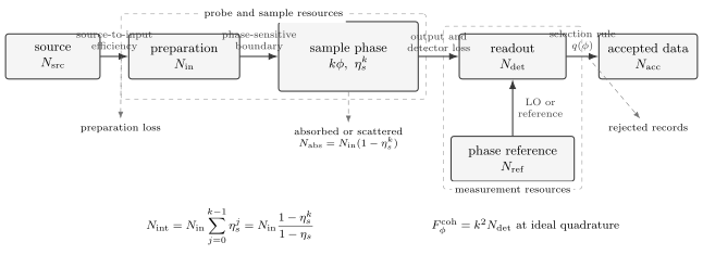
A resource ledger follows photons across physically distinct boundaries. Repeated sample interrogation increases the encoded phase to $k\phi$, but it also increases sample interactions and compounds transmission loss. A local oscillator or phase reference enters through a separate port and must be named whenever it changes the operational measurement.

For a sample with per-pass transmissivity $\eta_s$ and $k$ passes, a simple independent-loss model gives

$$\begin{aligned} N_{\mathrm{int}} &= N_{\mathrm{in}} \sum_{j=0}^{k-1}\eta_s^j = N_{\mathrm{in}} \frac{1-\eta_s^k}{1-\eta_s}, \\ N_{\mathrm{abs}} &= N_{\mathrm{in}}(1-\eta_s^k) = (1-\eta_s)N_{\mathrm{int}}. \end{aligned}$$

The model assumes that a photon surviving one pass is available for the next, that absorption events are independent, and that $\eta_s$ does not depend on the unknown phase. Saturable, nonlinear, bleaching, heating, or backaction- limited samples require a more detailed channel and damage functional.

The Phase Reference Is Part of the Experiment

Optical phase is relational. Without an external phase reference, coherences between different total-photon-number sectors are not operationally accessible. The appropriate state is then the globally phase-averaged state

$$\mathcal G(\rho) = \frac{1}{2\pi} \int_0^{2\pi} d\vartheta\, e^{-i\vartheta\hat N} \rho e^{i\vartheta\hat N}.$$

This $U(1)$ twirl removes matrix elements connecting different total-number sectors while preserving coherence between the two paths within each sector. The operational QFI must be calculated from $\mathcal G(\rho)$ if no suitable reference is present.

Consider a coherent state injected into one input port and vacuum into the other. After a balanced first beam splitter, the mean internal photon number is $\bar N$. For the differential generator $J_z$,

$$F_Q=4\operatorname{Var}(J_z)=\bar N.$$

The same value survives global phase averaging because every fixed-$N$ sector contains the relevant path coherence. In contrast, treating a one-arm phase as generated by $a^\dagger a$ before declaring a reference can yield an additional QFI contribution from number coherence. That contribution is usable only if a phase standard, such as a local oscillator, makes the corresponding common phase observable.

This distinction matters in two ways:

• a local oscillator need not be counted as probe dose if it never touches the sample, but its energy, stability, and mode quality remain instrument resources;
• a comparison between reference-free counting and reference-assisted homodyne detection must state which reference operations are free.

There is no universal rule that every reference photon must be added to the sample photon budget. The rule is to declare the boundary and use it consistently for every comparator.

Local Precision and Global Phase Risk

The Cramér–Rao framework describes local curvature of a likelihood near a specified phase. An optical phase is periodic, so a globally meaningful protocol must also resolve aliases. An ideal NOON measurement contains terms such as

$$p(x|\phi,\theta) \propto 1+(-1)^x\cos[N(\phi-\theta)],$$

which repeat every $2\pi/N$. The local slope is steep, but one observation does not identify which of the $N$ branches contains the true phase.

For a circular parameter, ordinary mean-squared error can depend on an arbitrary branch cut. Two useful alternatives are the periodic cost

$$c(\hat\phi,\phi) = 4\sin^2\!\left( \frac{\hat\phi-\phi}{2} \right)$$

and the Holevo variance

$$V_H = \left| \left\langle e^{i(\hat\phi-\phi)} \right\rangle \right|^{-2}-1.$$

A trustworthy global analysis specifies a prior on the circle, reports a Bayesian or minimax risk, and includes every coarse measurement or adaptive step used to select the final branch. Common strategies combine low-frequency and high-frequency fringes, vary the interrogation number $k$, or adapt $\theta$ from the current posterior. Bayes’ Rule provides the probability update; Cramér–Rao Bounds explains why a local bound alone does not settle this global problem.

Benchmark Probe Families

The following idealized families illuminate different tradeoffs. Their QFI values are not interchangeable performance claims.

Probe inside the interferometer	Ideal local information	Main strength	Main qualification
Independent balanced-path photons or coherent light	$F_Q=N$ or $\bar N$	Simple preparation and robust readout	Establishes the matched independent-photon baseline only after losses and references are fixed
Bright coherent field plus squeezed vacuum	$F_Q\sim N_c e^{2r}$ in the bright, ideal regime	Practical constant-factor noise reduction	Loss and squeezing-angle error mix anti-squeezed or vacuum noise into readout
NOON state	$F_Q=N^2$	Maximum fixed-$N$ generator variance	$N$-fold phase ambiguity and exponential fragility of its path coherence under loss
Twin-Fock input and Holland–Burnett state	$F_Q=N(N+2)/2$ for total even $N$	High ideal information with better loss behavior than NOON states in many regimes	Preparation and near-optimal number-resolving readout are demanding
A probe making $k$ coherent passes	$F_Q\propto k^2$ per surviving probe	Reuses preparation and detection hardware	Uses $k$ phase queries, narrows global range, takes time, and incurs compounded loss

Here $N_c$ is the bright coherent photon number and $r$ is the squeezing parameter. Exact squeezed-state formulas depend on where the resource boundary is placed and which mean photon numbers are fixed. The optical preparation and readout physics belong in Squeezed Light and Interferometers.

The Holland–Burnett entry begins with equal number states $|n,n\rangle$ at the input of a balanced beam splitter, with total photon number $N=2n$. The state inside the arms has

$$F_Q = 2n(n+1) = \frac{N(N+2)}{2}.$$

This is below the NOON value $N^2$ at large $N$ by a factor approaching two, but a lower ideal QFI can be a good trade when the resulting likelihood is more robust or experimentally accessible.

Loss Changes the Asymptotic Limit

Model pure loss in an arm by coupling the optical mode to an inaccessible environmental vacuum mode. If the environment can carry information about which path lost a photon, it destroys some of the coherence that encoded $\phi$. Tracing out that environment turns a pure probe into a mixture and reduces its QFI.

Loss location matters:

• source and preparation loss changes the state and $N_{\mathrm{in}}$;
• internal arm loss can reveal path information and changes the encoded state;
• sample absorption is both a noise mechanism and often the relevant cost;
• output and detector loss discards outcomes after encoding;
• reference-path loss degrades mode matching and phase readout.

One cannot in general combine these into a single efficiency and retain the same physical interpretation, even when a fitted visibility happens to agree.

For an ideal NOON state under equal independent transmissivity $\eta$ in its phase-sensitive paths, the coherence requiring all $N$ photons to survive is suppressed approximately as $\eta^N$. A useful local-information diagnostic is therefore

$$F_{\mathrm{NOON}} \sim N^2\eta^N,$$

before adding preparation and detection inefficiency. This expression is not a universal exact bound, but it displays the central fragility: increasing $N$ steepens the surviving fringe while exponentially reducing its occurrence.

More generally, in the standard symmetric pure-loss model with fixed transmissivity $0<\eta<1$, the asymptotic precision obeys a channel bound of the form

$$\Delta\phi \geq \sqrt{ \frac{1-\eta}{\eta N} }.$$

The precise finite-$N$ optimum and prefactor depend on the loss convention and allowed input class, but the scaling message is robust: fixed nonzero loss restores a $1/\sqrt N$ asymptote. Quantum probes may retain a valuable constant advantage, yet the ideal $1/N$ root-mean-square scaling does not persist to arbitrarily large $N$ through a fixed-loss channel. This is one reason bright coherent light plus squeezed vacuum can approach practically relevant optical bounds without requiring very large path-entangled number states.

For coherent light with $N$ photons incident before a phase-independent net efficiency $\eta$, a corresponding shot-noise benchmark is

$$\Delta\phi_{\mathrm{coh}} = \frac{1}{\sqrt{\eta N}}.$$

Comparing the two formulas shows that the asymptotic quantum improvement is a constant in $N$ under the stated channel model. It does not show that the bound is attained by a particular source, detector, and estimator.

Multipass Interferometry

If a surviving photon traverses the phase element $k$ times, it accumulates $k\phi$. For a coherent or independent-photon probe, the local FI per launched photon under per-pass transmission $\eta_s$ is ideally

$$f_{\mathrm{in}}(k) = k^2\eta_s^k.$$

The factor $k^2$ is the squared phase lever; $\eta_s^k$ is the survival probability. Calling this a free $k^2$ gain would omit both channel uses and loss. With $N_{\mathrm{in}}$ launched photons, the total number of ideal phase queries in the lossless case is

$$Q=kN_{\mathrm{in}}.$$

Sequential queries and simultaneous entanglement can realize related generator variances, so a fair Heisenberg-scaling statement counts every use of the unknown phase channel. Heisenberg Scaling develops this query-complexity viewpoint.

For a sample-limited comparison, divide the information by absorbed photons:

$$\frac{F_\phi}{N_{\mathrm{abs}}} = \frac{k^2\eta_s^k}{1-\eta_s^k}$$

for the simple coherent multipass model. Treating $k$ continuously, write $x=-k\ln\eta_s$. Maximizing $x^2/(e^x-1)$ gives

$$2(1-e^{-x})=x, \qquad x\simeq1.5936,$$

so the optimal surviving fraction is approximately

$$\eta_s^k=e^{-x}\simeq0.2032.$$

This is an illuminating benchmark, not a universal design prescription. Additional circulation loss, finite coherence time, detector saturation, sample dynamics, and a maximum allowed measurement time can move the optimum. It also shows why a single-pass coherent comparator can be too weak for a sample-damage claim: a well-designed classical multipass strategy already uses the sample much more efficiently.

Sample Dose and Disturbance

In microscopy, spectroscopy, and material characterization, available source power may be cheap while absorbed photons alter or destroy the sample. The relevant optimization is then information per disturbance, not information per detected photon.

For independent absorption with energy $\hbar\omega$ per lost photon, the expected deposited energy is approximately

$$E_{\mathrm{dep}} = \hbar\omega N_{\mathrm{abs}}.$$

Real samples may instead be limited by peak intensity, nonlinear absorption, heating rate, photochemical pathways, or the probability of any destructive event. A general task should therefore introduce a disturbance observable or cost $D$ and optimize a risk such as

$$\mathcal R = \mathbb E[c(\hat\phi,\phi)] + \lambda\mathbb E[D],$$

where $\lambda$ expresses the application’s tradeoff. This formulation prevents “dose” from becoming a vague synonym for whichever photon count makes a protocol look best.

A fair sample-limited comparison should match at least:

1. the prior phase range and estimator cost;
2. total sample interactions or a physically justified damage measure;
3. acquisition time and usable bandwidth;
4. source, preparation, and detection efficiencies;
5. allowed reference beams and ancillary modes;
6. failure, heralding, and postselection probabilities.

Quantum improvement can remain after this audit, but it is then a statement about a specified sensing task rather than about a fringe in isolation.

Common Phase and Other Nuisance Parameters

Let $\phi_c$ be a common optical phase and $\phi_d$ the differential phase. A convenient joint model is

$$U(\phi_c,\phi_d) = \exp\!\left[ -i\left( \frac{\phi_c\hat N}{2} + \phi_d J_z \right) \right].$$

Without an external reference, $\phi_c$ is unobservable. With one, common-mode phase noise, local-oscillator drift, and path mismatch can couple into the readout. Other nuisance parameters include visibility, both arm transmissivities, detector gain and dark counts, mode overlap, background light, and the phase-to-signal calibration coefficient.

For parameters $\boldsymbol\theta=(\phi,\boldsymbol\lambda)$, the relevant classical Fisher information is a matrix. If the nuisance block is invertible, the information remaining for $\phi$ after jointly fitting $\boldsymbol\lambda$ is the Schur complement

$$F_{\mathrm{eff}} = F_{\phi\phi} - F_{\phi\lambda} F_{\lambda\lambda}^{-1} F_{\lambda\phi}.$$

Thus

$$\operatorname{Var}(\hat\phi) \geq \frac{1}{F_{\mathrm{eff}}} \geq \frac{1}{F_{\phi\phi}}.$$

Calibrating a nuisance parameter in a separate data set does not make its uncertainty vanish; the calibration information or prior must enter the joint model. A phase sensitivity quoted after fixing visibility, loss, and reference phase at their fitted values is usually conditional and should be labeled as such.

Readout, Postselection, and Attainability

QFI is an upper bound over measurements. The achieved FI belongs to the actual record, including detector response and data rejection. Number-resolving detection can preserve information hidden by threshold detectors; homodyne detection supplies a quadrature reference; parity can be optimal for some ideal states but difficult at large photon number. Photon Counting and Homodyne and Heterodyne Detection own those measurement models.

Suppose a trial is accepted with probability $q(\phi)$ and its conditional accepted-data FI is $F_{\mathrm{acc}}$. If a rejected trial carries no further record, the full per-launch FI is

$$F_{\mathrm{full}} = qF_{\mathrm{acc}} + \frac{[\partial_\phi q]^2}{q(1-q)}.$$

When $q$ is phase independent, this reduces to $qF_{\mathrm{acc}}$. Reporting only $F_{\mathrm{acc}}$ treats failed trials as free and can manufacture an apparent advantage. When $q$ depends on phase, the accept/reject flag itself carries information and must remain in the likelihood.

Attainability also depends on the operating regime. A POVM that saturates QFI may depend on the unknown phase; adaptive feedback or a preliminary coarse estimate may be needed. Finite data can produce biased, multimodal, or boundary-limited estimates even when an asymptotic local bound is tight.

Worked Resource Audit

Suppose a source emits $10^6$ photons per trial. Preparation transmission is $\eta_{\mathrm{pre}}=0.8$, a sample has per-pass transmission $\eta_s=0.9$, each surviving photon makes $k=3$ passes, and output plus detector efficiency is $\eta_{\mathrm{post}}=0.7$. Then

$$N_{\mathrm{in}} = 0.8\times10^6 = 8.0\times10^5.$$

The sample ledger is

$$\begin{aligned} N_{\mathrm{int}} &= (8.0\times10^5)(1+0.9+0.9^2) \\ &= 2.168\times10^6, \\ N_{\mathrm{abs}} &= (8.0\times10^5)(1-0.9^3) \\ &= 2.168\times10^5, \\ N_{\mathrm{det}} &= (8.0\times10^5)(0.9^3)(0.7) \\ &= 4.0824\times10^5. \end{aligned}$$

For ideal independent-photon readout at quadrature, each detected photon sees phase $3\phi$, so

$$F_\phi = k^2N_{\mathrm{det}} = 3.67416\times10^6.$$

The local shot-noise uncertainty is therefore

$$\Delta\phi \geq \frac{1}{\sqrt{F_\phi}} \simeq 5.22\times10^{-4}\,\mathrm{rad}.$$

This is a conditional model result, not yet an instrument specification. It assumes known efficiencies, unit visibility, no phase drift, no detector background, a locally known branch of a $2\pi/3$-periodic likelihood, and no extra circulation time or loss.

What Different Claims Establish

Evidence for optical quantum advantage comes in levels. Each level is useful, but they answer different questions.

Claim	What must be shown	What it does not yet establish
Nonclassical state preparation	A calibrated witness, tomography, squeezing, or sub-Poissonian statistic	Better phase estimation
Phase super-resolution	Fringes oscillate faster than a one-pass classical fringe	Lower estimation error or better resource efficiency
Conditional sub-shot-noise readout	Accepted records have variance below a stated shot-noise model	Advantage per launched photon or per unit time
Fisher-information advantage	Measured likelihood gives more FI than a matched comparator	Globally reliable estimation or lower sample damage
End-to-end sensitivity advantage	The complete estimator beats a matched classical protocol with uncertainty coverage	Better performance for every application or cost function
Task-level utility	The relevant scientific or engineering loss improves under real constraints	A universal quantum advantage

An end-to-end report should publish enough information to reconstruct the claim: raw outcome categories, trial count, acceptance rule, likelihood or estimator, prior or capture range, resource ledger, loss placement, calibration uncertainty, confidence or credible interval construction, and the classical comparator. Error bars obtained only from a local curvature fit should not be presented as global phase certainty.

Common Mistakes

• Calling a narrow $N\phi$ fringe a sensitivity improvement without counting its $N$ aliases.
• Comparing a nonclassical experiment normalized by detected photons with a classical benchmark normalized by incident photons.
• Correcting for detector loss in the plotted sensitivity as though the lost outcomes had been observed.
• Treating heralding or postselection failures as free trials.
• Using $e^{-i\phi a^\dagger a}$ for an indefinite-number state without saying whether an external phase reference exists.
• Counting a $k$-pass probe once when the claimed resource is use of the unknown channel.
• Comparing a quantum single-pass protocol only with a classical single-pass protocol when classical multipass sensing is allowed.
• Combining preparation, sample, arm, and detector losses into one efficiency while making a claim about sample dose.
• Quoting QFI without identifying a realizable measurement or the operating point needed to approach it.
• Using $1/N$ local scaling from an ideal state as evidence for asymptotic performance through fixed nonzero loss.
• Ignoring phase-reference photons, stability, or mode matching when the reference changes which phase is observable.
• Reporting a conditional precision after fitting nuisance parameters as if those parameters were known exactly.

Exercises

1. Independent photons and a NOON state

For fixed total photon number $N$, calculate the QFI for (a) $N$ independent photons, each in an equal path superposition, and (b) a NOON state. State the local uncertainty scaling after $\nu$ independent repetitions.

Solution

For one balanced-path photon, $\operatorname{Var}(J_z)=1/4$, so $N$ independent photons have

$$F_Q^{\mathrm{ind}}=N.$$

The NOON state is an equal superposition of the extremal eigenvalues $J_z=\pm N/2$, hence

$$\operatorname{Var}(J_z)=\frac{N^2}{4}, \qquad F_Q^{\mathrm{NOON}}=N^2.$$

For $\nu$ independent repetitions, QFI adds. The local quantum Cramér–Rao bounds are

$$\Delta\phi_{\mathrm{ind}} \geq \frac{1}{\sqrt{\nu N}}, \qquad \Delta\phi_{\mathrm{NOON}} \geq \frac{1}{N\sqrt\nu}.$$

The second result presumes a known local branch and an attainable measurement.

2. Visibility and the operating point

Starting from

$$p_\pm = \frac{1\pm V\cos\delta}{2}, \qquad \delta=\phi-\theta,$$

derive the single-photon FI and find its value at quadrature.

Solution

The derivatives are

$$\partial_\phi p_\pm = \mp\frac{V\sin\delta}{2}.$$

Therefore

$$\begin{aligned} F_1 &= \sum_{s=\pm} \frac{(\partial_\phi p_s)^2}{p_s} \\ &= \frac{V^2\sin^2\delta} {1-V^2\cos^2\delta}. \end{aligned}$$

At $\delta=\pi/2$, $F_1=V^2$. Visibility reduces the best local FI quadratically in this effective likelihood.

3. Loss-limited NOON size

Use the diagnostic $F_{\mathrm{NOON}}\sim N^2\eta^N$. Determine the continuous $N$ that maximizes FI per incident photon, $F/N$, for $\eta=0.9$.

Solution

The information per incident photon scales as

$$g(N)=N\eta^N.$$

Taking a logarithm,

$$\frac{d}{dN}\ln g = \frac1N+\ln\eta.$$

The continuous optimum is

$$N_* = -\frac{1}{\ln\eta}.$$

For $\eta=0.9$,

$$N_* \simeq 9.49.$$

An actual fixed-number protocol compares nearby integers and includes all other efficiencies. The calculation illustrates that loss creates a finite optimal entangled size; larger is not automatically better.

4. Optimal classical multipass survival

For a coherent multipass protocol, maximize

$$h(k) = \frac{k^2\eta^k}{1-\eta^k}$$

with respect to continuous $k$. Show that the optimal survival probability is independent of $\eta$.

Solution

Set $x=-k\ln\eta$, so $\eta^k=e^{-x}$. Apart from the constant $1/(\ln\eta)^2$,

$$h(x) \propto \frac{x^2}{e^x-1}.$$

The stationary condition is

$$2(e^x-1)-xe^x=0,$$

or

$$2(1-e^{-x})=x.$$

The nonzero solution is $x\simeq1.5936$, giving

$$\eta^{k_*} = e^{-x} \simeq 0.2032.$$

Thus the simple ideal model chooses $k$ so roughly $20\%$ of launched photons survive the sample, regardless of the per-pass transmission. Integer $k$ and apparatus losses modify the practical choice.

5. A three-pass photon ledger

Let $N_{\mathrm{src}}=2.0\times10^5$, $\eta_{\mathrm{pre}}=0.75$, $\eta_s=0.8$, $k=3$, and $\eta_{\mathrm{post}}=0.6$. Find $N_{\mathrm{in}}$, $N_{\mathrm{int}}$, $N_{\mathrm{abs}}$, and $N_{\mathrm{det}}$.

Solution

First,

$$N_{\mathrm{in}} = (2.0\times10^5)(0.75) = 1.5\times10^5.$$

Then

$$\begin{aligned} N_{\mathrm{int}} &= (1.5\times10^5)(1+0.8+0.8^2) \\ &= 3.66\times10^5, \\ N_{\mathrm{abs}} &= (1.5\times10^5)(1-0.8^3) \\ &= 7.32\times10^4, \\ N_{\mathrm{det}} &= (1.5\times10^5)(0.8^3)(0.6) \\ &= 4.608\times10^4. \end{aligned}$$

Notice that the interaction count exceeds the launched count, whereas the detected count is much smaller. Each answers a different resource question.

6. Postselection accounting

A heralded protocol accepts a phase-independent fraction $q=0.04$ of trials. Accepted records have $F_{\mathrm{acc}}=100$ per accepted trial. Find the FI per launched trial. Compare it with a deterministic protocol having FI $5$ per trial.

Solution

Because $q$ is phase independent,

$$F_{\mathrm{full}} = qF_{\mathrm{acc}} = (0.04)(100) = 4.$$

The accepted subset looks twenty times more informative than the deterministic record, but the complete heralded protocol has less FI per launch: $4<5$. This does not make heralding useless; it shows that its success probability belongs in the chosen resource normalization.

7. Nuisance-parameter penalty

Suppose the Fisher matrix for phase $\phi$ and visibility $V$ is

$$F = \begin{pmatrix} 100 & 18\\ 18 & 9 \end{pmatrix}.$$

Find the effective phase information when $V$ is estimated jointly, and compare the resulting bound with the bound obtained by incorrectly treating $V$ as known.

Solution

The Schur complement is

$$F_{\mathrm{eff}} = 100-18(9^{-1})18 = 64.$$

Thus

$$\Delta\phi \geq \frac1{\sqrt{64}} = 0.125.$$

Treating $V$ as known would give $1/\sqrt{100}=0.1$. Correlation with the uncertain visibility weakens the attainable phase precision.

8. Audit a quantum-advantage claim

An experiment reports a NOON fringe with period $2\pi/6$ and a conditional phase variance below the coherent shot-noise level calculated from the six detected photons in each accepted event. List at least six additional facts needed to establish an end-to-end sensing advantage.

Solution

A sufficient audit would ask for at least:

1. the prior or capture range and a procedure for resolving the six aliases;
2. source photons or trials per accepted event;
3. preparation, heralding, transmission, and detector efficiencies;
4. the full likelihood including rejected and zero-count outcomes;
5. the estimator and uncertainty-coverage validation;
6. acquisition time and bandwidth;
7. phase-reference resources and stability;
8. a classical comparator allowed the same multipass, adaptive, and reference operations;
9. sample interactions or absorbed photons if damage matters;
10. calibration and nuisance-parameter uncertainties.

The observed fringe establishes phase super-resolution and may establish nonclassical coherence. It does not by itself establish more information per launch, per unit time, or per absorbed photon.

References

1. C. M. Caves, “Quantum-mechanical noise in an interferometer,” Physical Review D 23, 1693–1708 (1981), doi:10.1103/PhysRevD.23.1693.
2. B. Yurke, S. L. McCall, and J. R. Klauder, “SU(2) and SU(1,1) interferometers,” Physical Review A 33, 4033–4054 (1986), doi:10.1103/PhysRevA.33.4033.
3. M. J. Holland and K. Burnett, “Interferometric detection of optical phase shifts at the Heisenberg limit,” Physical Review Letters 71, 1355–1358 (1993), doi:10.1103/PhysRevLett.71.1355.
4. S. L. Braunstein and C. M. Caves, “Statistical distance and the geometry of quantum states,” Physical Review Letters 72, 3439–3443 (1994), doi:10.1103/PhysRevLett.72.3439.
5. D. W. Berry and H. M. Wiseman, “Optimal states and almost optimal adaptive measurements for quantum interferometry,” Physical Review Letters 85, 5098–5101 (2000), doi:10.1103/PhysRevLett.85.5098.
6. B. L. Higgins, D. W. Berry, S. D. Bartlett, H. M. Wiseman, and G. J. Pryde, “Entanglement-free Heisenberg-limited phase estimation,” Nature 450, 393–396 (2007), doi:10.1038/nature06257.
7. R. Demkowicz-Dobrzański, U. Dorner, B. J. Smith, J. S. Lundeen, W. Wasilewski, K. Banaszek, I. A. Walmsley, “Quantum phase estimation with lossy interferometers,” Physical Review A 80, 013825 (2009), doi:10.1103/PhysRevA.80.013825.
8. M. Jarzyna and R. Demkowicz-Dobrzański, “Quantum interferometry with and without an external phase reference,” Physical Review A 85, 011801(R) (2012), doi:10.1103/PhysRevA.85.011801.
9. M. J. W. Hall and H. M. Wiseman, “Does nonlinear metrology offer improved resolution? Answers via quantum information theory,” Physical Review X 2, 041006 (2012), doi:10.1103/PhysRevX.2.041006.
10. R. Demkowicz-Dobrzański, J. Kołodyński, and M. Guță, “The elusive Heisenberg limit in quantum-enhanced metrology,” Nature Communications 3, 1063 (2012), doi:10.1038/ncomms2067.
11. R. Demkowicz-Dobrzański, M. Jarzyna, and J. Kołodyński, “Quantum limits in optical interferometry,” Progress in Optics 60, 345–435 (2015), doi:10.1016/bs.po.2015.02.003.
12. M. A. Taylor and W. P. Bowen, “Quantum metrology and its application in biology,” Physics Reports 615, 1–59 (2016), doi:10.1016/j.physrep.2015.12.002.
13. R. Schnabel, “Squeezed states of light and their applications in laser interferometers,” Physics Reports 684, 1–51 (2017), doi:10.1016/j.physrep.2017.04.001.
14. P. M. Birchall, J. L. O’Brien, J. C. F. Matthews, and H. Cable, “Quantum-classical boundary for precision optical phase estimation,” Physical Review A 96, 062109 (2017), doi:10.1103/PhysRevA.96.062109.
15. L. Pezzè, A. Smerzi, M. K. Oberthaler, R. Schmied, and P. Treutlein, “Quantum metrology with nonclassical states of atomic ensembles,” Reviews of Modern Physics 90, 035005 (2018), doi:10.1103/RevModPhys.90.035005.

Further Connections

• Interferometers derives the optical Mach–Zehnder transformation, count likelihoods, squeezed-input response, readout methods, calibration, and physical applications.
• Beam Splitters owns two-port unitary conventions and photon interference at the individual optical element.
• Quantum Measurement as Estimation provides the estimand, likelihood, estimator, risk, and validation framework used here.
• Classical and Quantum Fisher Information develops score information, QFI, data-processing bounds, and attainability.
• Standard Quantum Limit defines matched independent-probe baselines and explains why “shot noise” must name a resource boundary.
• Heisenberg Scaling treats generator range, phase queries, global ambiguity, fluctuating resources, and noisy asymptotes.
• Squeezing develops covariance ellipses and the metrological meaning of reduced quadrature noise.
• Noise and Decoherence in Metrology derives the fixed-loss asymptotic phase bound and explains why fragile noiseless optima need not remain optimal under loss.
• Erasure and Loss Channels gives channel representations and operational distinctions between flagged erasure and unobserved loss.
• Photonic Qubits places path encoding, sources, interferometric control, and detectors in a hardware stack.