Distributed Quantum Sensing

Distributed quantum sensing uses quantum states or quantum correlations shared among spatially separated sensor nodes to estimate a declared property of a field, signal, or set of local parameters. A network might estimate the average phase across several optical paths, a frequency difference between remote clocks, a magnetic-field gradient, or one spatial mode of a fluctuating field. The target is often a weighted functional

$$q := \mathbf w^{\mathsf T}\boldsymbol\theta = \sum_{m=1}^{M}w_m\theta_m,$$

where $\theta_m$ is the response accumulated at node $m$ and $\mathbf w$ defines the spatial mode of interest.

The phrase does not mean merely operating several quantum sensors. Independent quantum sensors followed by classical averaging already form a distributed sensor system. A specifically distributed quantum advantage requires a matched comparison showing that inter-node quantum resources improve the declared network task beyond the best allowed node-separable protocol. The comparison must include local nonclassical resources when those are allowed, not only coherent states or independent particles.

Entanglement is strongly task-dependent. It can directly concentrate information into a global functional such as an average. It need not improve, and can even obstruct, reconstruction of every local parameter. Loss at one node can erase a global correlation, and a shared oscillator, synchronized control, accepted-shot rule, or high-power local oscillator may dominate the real resource ledger. The right question is therefore not whether a network is entangled, but whether its complete estimator gains information about the specified spacetime mode per matched resource and per unit wall time.

Canonical Scope

Quantum Network Architectures owns entanglement services, physical and logical topologies, routing, scheduling, memories, reference-frame metadata, and network control planes. Network Verification owns source and device trust, test-versus-use sampling, topology tests, and service certification. Those topics are used here rather than rebuilt as a network stack.

Classical and Quantum Fisher Information owns Fisher matrices, symmetric logarithmic derivatives, multiparameter compatibility, and attainability. Standard Quantum Limit and Heisenberg Scaling own the general independent-probe and ideal collective scaling laws. GHZ States, Squeezing, and Spin Squeezing own the underlying state families and their local metrological properties.

This page owns the synthesis specific to sensing across nodes:

• the distinction between estimating a field map and estimating one global field functional;
• the local-encoding model and network identifiability conditions;
• matched product-probe, node-separable, and inter-node-entangled benchmarks;
• discrete-variable and continuous-variable distributed protocols;
• covariance-mode engineering and rejection of structured nuisance fields;
• link loss, state age, timing, reference frames, acceptance, and wall-time information rate; and
• the evidence required to claim a distributed quantum advantage.

Complete clock, magnetometer, inertial-sensor, and optical-interferometer hardware remains in the corresponding platform pages. The focus here is the network estimation problem that begins after local couplings have been specified.

Define the Network Task

Local responses are filtered field samples

A sensor does not read an instantaneous field value at a mathematical point. Let $s(\mathbf x,t)$ be a physical field and let node $m$ have position $\mathbf x_m$, calibrated temporal response $h_m(t)$, and coupling coefficient $\kappa_m$. Its dimensionless encoded parameter can be written

$$\theta_m := \kappa_m \int_{-\infty}^{\infty} h_m(t) s(\mathbf x_m,t) \,\mathrm dt.$$

Finite sensor volume can be included by replacing the point sample with a spatial integral. Clock interrogation windows, interferometer sensitivity functions, dynamical-decoupling filters, and optical transit times all enter through $h_m$. A network therefore samples a collection of spacetime modes, not an abstract vector detached from hardware.

The target might be:

• a normalized average, $q=M^{-1}\sum_m\theta_m$;
• a difference, $q=(\theta_1-\theta_2)/2$;
• a finite-difference gradient or curvature;
• a matched filter for a predicted spatial profile;
• one coefficient in a basis expansion of a field; or
• the full vector $\boldsymbol\theta$.

These are different statistical problems. A state optimized for the average may deliberately contain little information about differences. It cannot then be credited with high-resolution imaging of all nodes.

The local encoding model

For $M$ nodes with locally acting generators $G_m$, a standard phase model is

$$U_{\boldsymbol\theta} = \bigotimes_{m=1}^{M} \exp\!\left(-i\theta_mG_m\right).$$

Operators at distinct nodes commute because they act on distinct tensor factors. The input state need not factorize: it may contain particle entanglement within each node, mode entanglement among nodes, or both. After the local interactions, measurements may be local with classical post-processing or genuinely joint. Which operations are allowed is part of the comparison.

For a parameter vector, a measurement produces a Fisher matrix $\mathbf F_{\theta}$. If all components are locally identifiable and an unbiased estimator is used in the regular asymptotic regime, then estimating $q=\mathbf w^{\mathsf T}\boldsymbol\theta$ through the vector model gives

$$\operatorname{Var}(\widehat q) \geq \frac{1}{\nu} \mathbf w^{\mathsf T} \mathbf F_{\theta}^{-1} \mathbf w,$$

for $\nu$ independent repetitions. A generalized inverse and explicit identifiability constraints are required when $\mathbf F_{\theta}$ is singular.

This expression should not be confused with $\mathbf w^{\mathsf T}\mathbf F_{\theta}\mathbf w$. If the physics instead contains only one unknown $q$ through $\boldsymbol\theta=\mathbf vq$, then

$$F_q = \mathbf v^{\mathsf T} \mathbf F_{\theta} \mathbf v.$$

The first problem treats orthogonal field modes as unknown nuisance parameters. The second assumes they are absent or known. Switching between them can change a claimed quantum advantage.

A minimum sensing contract

Before comparing protocols, state at least:

Item	Required declaration
estimand	full local vector, weighted functional, field-model coefficient, or detection decision
local response	positions, coupling gains, generators, temporal filters, and sign conventions
nuisance model	unknown offsets, gradients, oscillator phase, link phase, drift, and environmental modes
quantum boundary	product particles, local entanglement, inter-node entanglement, memories, and reference modes allowed
resource boundary	particles or photons launched, interacting, surviving, and detected; source and link attempts
timing	simultaneous window, allowed latency, cycle time, dead time, and state age
measurement	local or joint POVM, classical communication, accepted outcomes, and estimator
objective	local variance, Bayesian risk, hypothesis error, Fisher information rate, or time to target
validation	calibration data, matched comparator, independent checks, and uncertainty statement

Without this contract, phrases such as “network SQL” or “Heisenberg scaling with node number” are underdetermined. Adding nodes can add probes, spatial coverage, source brightness, reference beams, or interrogation time. Those are different resources.

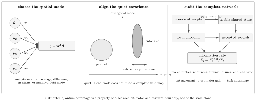
Distributed sensing begins by selecting a weighted spatial mode $q=\mathbf w^{\mathsf T}\boldsymbol\theta$. Product probes, node-local entanglement, and inter-node entanglement have different matched benchmarks. Any gain must survive state distribution, local encoding, readout, accepted outcomes, and cycle-time accounting.

Covariance Geometry

Suppose calibrated local readouts obey

$$\mathbf y = \boldsymbol\theta + \boldsymbol\varepsilon, \qquad \mathbb E[\boldsymbol\varepsilon] = \mathbf0,$$

with noise covariance $\boldsymbol\Sigma$. The linear estimator $\widehat q=\mathbf w^{\mathsf T}\mathbf y$ has

$$\operatorname{Var}(\widehat q) = \mathbf w^{\mathsf T} \boldsymbol\Sigma \mathbf w.$$

Distributed quantum resources are useful when they reduce this quadratic form for the target mode. Negative cross-covariances can quiet an average; positive cross-covariances can quiet a difference. A covariance ellipse squeezed along one direction must generally broaden along another, so the target weights must be chosen before the state is optimized.

The same formula also describes classical correlations. Synchronous interrogation with a common oscillator can reject oscillator noise in a difference, and subtracting a shared auxiliary sensor can create correlated residuals. Observing $\mathbf w^{\mathsf T}\boldsymbol\Sigma\mathbf w$ below the sum of individual variances is therefore not an entanglement witness. A quantum claim needs a state or channel certificate and a bound satisfied by every allowed node-separable protocol.

Nuisance-mode rejection

Suppose local phases follow a known linear field model

$$\boldsymbol\theta = \mathbf A\boldsymbol\beta,$$

where columns of $\mathbf A$ contain sampled spatial profiles and $\boldsymbol\beta$ contains their unknown amplitudes. To estimate coefficient $\beta_s$ without bias, weights must satisfy

$$\mathbf A^{\mathsf T}\mathbf w = \mathbf e_s.$$

Among linear unbiased estimators, the minimum-variance weights are

$$\mathbf w_\star = \boldsymbol\Sigma^{-1}\mathbf A \left( \mathbf A^{\mathsf T} \boldsymbol\Sigma^{-1} \mathbf A \right)^{-1} \mathbf e_s,$$

provided the indicated matrices have the required rank. Quantum correlations can reshape $\boldsymbol\Sigma$, but they cannot recover a field component that the sampled response matrix does not identify. Geometry and calibration come before squeezing.

Three Different Resource Benchmarks

The cleanest hierarchy appears in a normalized qubit-phase model. Assume:

• $N$ two-level probes are distributed among $M$ nodes;
• each probe samples its local phase once through a generator with eigenvalue span one;
• all local phases not fixed by the estimand may be unknown;
• control, contrast, detection, and prior knowledge are ideal; and
• the experiment is repeated independently $\nu$ times.

These assumptions define an illustrative bound, not a universal law for every sensor network.

Independent product probes

Let node $m$ receive $n_m$ independent probes, with $\sum_m n_m=N$. Its local Fisher information is at most $n_m$ in this normalization. Independent local estimates give

$$\operatorname{Var}(\widehat q) \geq \frac{1}{\nu} \sum_{m=1}^{M} \frac{w_m^2}{n_m}.$$

Optimizing the allocation under the fixed total yields

$$n_m = N \frac{|w_m|}{\|\mathbf w\|_1}, \qquad \operatorname{Var}(\widehat q)_{\rm prod} \geq \frac{\|\mathbf w\|_1^2}{\nu N},$$

where

$$\|\mathbf w\|_1 := \sum_m|w_m|.$$

Equal allocation is optimal only for equal-magnitude weights. Sending the same number of probes to a nearly irrelevant node wastes the declared resource.

Node-separable states with local entanglement

A stronger comparator allows arbitrary entanglement among the $n_m$ probes inside each node but no entanglement between nodes. An ideal local GHZ-like state can provide Fisher information $n_m^2$ for $\theta_m$, giving

$$\operatorname{Var}(\widehat q) \geq \frac{1}{\nu} \sum_{m=1}^{M} \frac{w_m^2}{n_m^2}.$$

The optimized allocation is now

$$n_m = N \frac{|w_m|^{2/3}}{ \sum_j|w_j|^{2/3} },$$

and therefore

$$\operatorname{Var}(\widehat q)_{\rm node\text{-}sep} \geq \frac{ \left( \sum_m|w_m|^{2/3} \right)^3 }{ \nu N^2 }.$$

This is the appropriate ideal benchmark when each node may prepare its own nonclassical ensemble. Beating the product-probe SQL while remaining above this bound demonstrates quantum enhancement, but not an advantage due specifically to entanglement between nodes.

Inter-node entanglement

A signed GHZ-type state can place the entire weighted functional into one collective phase. Allocate

$$n_m = N \frac{|w_m|}{\|\mathbf w\|_1}$$

and reverse the local coupling for negative $w_m$. The relative phase between the two GHZ branches is

$$\Phi = \sum_m \operatorname{sgn}(w_m)n_m\theta_m = \frac{N}{\|\mathbf w\|_1} q.$$

An ideal parity measurement then gives

$$\operatorname{Var}(\widehat q)_{\rm global} \geq \frac{\|\mathbf w\|_1^2}{\nu N^2}.$$

For arbitrary real weights, finite $N$ may require rounded allocations or a sequence of settings whose average realizes the desired coefficients. The bound also assumes local controls can implement the required signs and that orthogonal field modes are allowed to remain unestimated.

For an equal average, $w_m=1/M$, the hierarchy becomes

$$\begin{aligned} \operatorname{Var}(\widehat q)_{\rm prod} &\geq \frac{1}{\nu N}, \\ \operatorname{Var}(\widehat q)_{\rm node\text{-}sep} &\geq \frac{M}{\nu N^2}, \\ \operatorname{Var}(\widehat q)_{\rm global} &\geq \frac{1}{\nu N^2}. \end{aligned}$$

The factor $M$ between the last two variances is the ideal advantage of inter-node entanglement over separately entangled nodes for this particular global task. It is not a generic advantage for estimating all $M$ phases.

What must be matched

A defensible comparison uses the same:

• field functional and nuisance model;
• number of probes that actually sample each location;
• interrogation time and number of field interactions;
• source attempts, state-preparation success, and accepted-shot rule;
• local oscillator, reference beams, ancillas, and memories;
• loss, detector capability, and classical communication;
• cycle time and total observation time; and
• prior range, branch-resolution strategy, and estimator.

A network may have a practical source-count advantage even without a better probe-count bound. For example, splitting one squeezed optical mode among nodes can replace $M$ independent squeezers. That is valuable engineering, but it should be reported separately from precision scaling at fixed photons incident on the samples.

Global Function Versus Full Field Map

For commuting local generators and a cost that asks for all local parameters, inter-node entanglement has no generic precision advantage. Broad classes of network problems admit optimal sensor-separable states and local measurements. For noncommuting generators, any intrinsic network advantage is still constrained by multiparameter incompatibility and can be modest.

The situation changes when only one global function is required. A GHZ or collective squeezed mode can spend nearly all available sensitivity on $q=\mathbf w^{\mathsf T}\boldsymbol\theta$ while discarding information about orthogonal combinations. That concentration is precisely why it can beat a strategy that separately learns every $\theta_m$ before combining them.

This yields a useful design rule:

Entangle across nodes only after deciding which spatial mode may be sacrificed and which one must be measured.

If the application later asks for a different weighting, the state, distribution network, local controls, or measurement basis may need to be reconfigured. One scalar network output cannot be retrospectively promoted to a complete field image.

Discrete-Variable Protocols

Signed GHZ sensing

For qubit or effective-spin nodes, the ideal global protocol prepares a coherence between two many-body branches. Local basis flips can reverse the sign with which selected probes accumulate phase. After encoding, the state has the form

$$|\psi(q)\rangle = \frac{1}{\sqrt2} \left( |\mathbf0\rangle + e^{-iK_qq} |\mathbf1\rangle \right), \qquad K_q = \frac{N}{\|\mathbf w\|_1}.$$

The strings $|\mathbf0\rangle$ and $|\mathbf1\rangle$ summarize the two signed branches; they need not be all-zero and all-one strings in the laboratory basis. An analysis rotation followed by local binary measurements produces a parity likelihood

$$p(\pi\mid q) = \frac12 \left[ 1 + \pi C \cos(K_qq+\phi_0) \right], \qquad \pi\in\{-1,+1\},$$

where $C$ is the final network contrast and $\phi_0$ is a controlled analysis phase. The classical Fisher information is

$$F_q = \frac{ C^2K_q^2 \sin^2(K_qq+\phi_0) }{ 1-C^2 \cos^2(K_qq+\phi_0) }.$$

At a quadrature working point,

$$F_q = C^2K_q^2.$$

Reduced projection noise alone is not enough: contrast determines the signal slope. A protocol with a narrow parity distribution and nearly vanishing contrast carries little phase information.

The parity can be assembled from local measurement records after classical communication. The sensor qubits need not be physically reunited after encoding. This does not enable faster-than-light signaling: no node can infer the global parity or the distant parameter from its local record alone.

Phase aliases and adaptive tiers

The same factor $K_q$ that increases local slope also shortens the fringe period:

$$q \sim q + \frac{2\pi}{K_q}.$$

An ideal $N$-probe global state therefore has a local uncertainty of order $1/N$ but an unambiguous interval of the same order. A broad prior requires a coarse product-state estimate, several interrogation strengths, adaptive analysis phases, or a Bayesian protocol that retains all branches. Quoting the local Fisher information while assuming the correct fringe index is known does not establish globally accurate sensing.

Split spin-squeezed ensembles

Atomic protocols can create correlations in one ensemble and then divide the atoms into spatial modes. Let $J_{z,m}$ be a local population-difference readout and let

$$\Gamma_{mn} := \frac12 \left\langle \Delta J_{z,m}\Delta J_{z,n} + \Delta J_{z,n}\Delta J_{z,m} \right\rangle.$$

For a calibrated linear response vector $\mathbf r_q$, an estimator using coefficients $\mathbf a$ obeys

$$\Delta q^2 = \frac{ \mathbf a^{\mathsf T} \boldsymbol\Gamma \mathbf a }{ |\mathbf a^{\mathsf T}\mathbf r_q|^2 }.$$

Mode entanglement appears through the off-diagonal blocks of $\boldsymbol\Gamma$. It is useful only when the quiet covariance direction is aligned with the desired average or difference and the full response slope is retained. Particle entanglement within the original ensemble and mode entanglement among the separated outputs are related but distinct statements.

A network claim must compare the split state with independently optimized local squeezed ensembles when those are physically allowed. Comparing only with coherent-spin states establishes sub-projection-noise operation, not necessarily an inter-node advantage.

Continuous-Variable Protocols

Squeeze the target supermode

Optical and microwave networks often encode weak signals as quadrature displacements or small phase rotations. Choose normalized real mode coefficients $u_m$ with $\sum_m u_m^2=1$ and define

$$X_{\mathbf u} := \sum_{m=1}^{M}u_mX_m.$$

A passive splitter network can distribute one squeezed input so that this collective output quadrature inherits the squeezing:

$$\operatorname{Var}(X_{\mathbf u}) = \frac12e^{-2r}$$

in the convention where vacuum variance is $1/2$. Orthogonal combinations of the node quadratures contain vacuum noise. Thus each local marginal can look only weakly squeezed while the correctly weighted sum recovers the quiet input mode.

Suppose local transducers produce

$$\mathbb E[X_m] = g_m\theta_m.$$

The homodyne weights and splitter amplitudes must be chosen so that the collective response is proportional to $q=\sum_mw_m\theta_m$. Unequal transducer gains, link attenuation, or local oscillator phases rotate the realized mode away from $\mathbf w$. Calibration must therefore determine the response vector, not merely the optical splitting ratios.

The correct separable optical comparator

A coherent-state network supplies the familiar shot-noise baseline, but it is not always the strongest separable comparator. If local squeezers are allowed, each node can receive its own optimized squeezed state. The comparison must then fix:

• photons incident on each sample or transducer;
• coherent displacement and squeezed-vacuum photons;
• source-to-sample transmission;
• local-oscillator and reference power when operationally relevant;
• detector efficiency and bandwidth; and
• the number and quality of nonclassical sources.

Distributing one squeezed source can outperform $M$ separable squeezed inputs at fixed total source photons, or it can offer similar sensitivity with fewer squeezers. Those are legitimate but different resource statements. A result should say whether the gain is per sample photon, per generated nonclassical photon, per source, or per wall-clock second.

Structured Noise and Protected Modes

Spatially correlated noise need not have the same profile as the signal. This creates an opportunity beyond simply reducing white projection noise. Let the Hamiltonian during interrogation be

$$H = \beta_s \sum_m s_mG_m + \sum_{\mu=1}^{K} \beta_\mu \sum_m n_{\mu m}G_m,$$

where $\mathbf s$ is the sampled signal profile and the vectors $\mathbf n_\mu$ are nuisance profiles. A coherence whose two branches differ by generator vector $\mathbf k$ accumulates relative phase

$$\Phi = t \left[ \beta_s\mathbf k^{\mathsf T}\mathbf s + \sum_{\mu=1}^{K} \beta_\mu \mathbf k^{\mathsf T}\mathbf n_\mu \right].$$

If

$$\mathbf k^{\mathsf T}\mathbf n_\mu = 0 \quad \text{for every }\mu, \qquad \mathbf k^{\mathsf T}\mathbf s \ne 0,$$

then the encoded coherence lies in a decoherence-free mode for those nuisance fields while retaining signal response. Multilevel sensors can supply a richer set of branch differences $\mathbf k$ than two-level sensors.

This protection is model-based. It fails when the nuisance profile is misspecified, node positions drift, coupling gains change, or unmodeled noise has a component along $\mathbf k$. A serious experiment measures the residual transfer from every rejected mode and propagates profile uncertainty into the final estimate.

Loss, Decoherence, and State Age

Discrete-variable survival

A global GHZ coherence is fragile because every participating subsystem is part of the signal-bearing off-diagonal term. If probe $j$ survives with probability $\eta_j$ and any loss causes rejection, then

$$p_{\rm surv} = \prod_{j=1}^{N}\eta_j.$$

If each probe also retains coherence amplitude $c_j$, the final contrast is bounded schematically by

$$C_{\rm net} \lesssim C_0 \prod_{j=1}^{N}c_j.$$

The conditional Fisher information may still scale as $C_{\rm net}^2N^2$, but the unconditional information per attempt is reduced by survival and preparation probability. Independent probes degrade gradually because lost probes can simply cease contributing; a monolithic GHZ state can lose its entire collective advantage after one erasure.

Heralded generation changes what is known, not what it costs. A failed link attempt may be excluded from the estimator only if its elapsed time, source uses, memory aging, and any consumed probes remain in the resource ledger.

Continuous-variable loss

For quadratures with vacuum covariance $I/2$, independent pure-loss channels transform a covariance matrix as

$$\boldsymbol V_{\rm out} = \boldsymbol L \boldsymbol V_{\rm in} \boldsymbol L + \frac12 \left( I-\boldsymbol L^2 \right),$$

where

$$\boldsymbol L = \operatorname{diag} \left( \sqrt{\eta_1},\ldots,\sqrt{\eta_M} \right)$$

for one quadrature per node. Loss injects independent vacuum noise and also distorts the target supermode when the $\eta_m$ differ. The optimum splitter and electronic weights in a lossy network need not equal their lossless values. At fixed nonzero loss, ideal Heisenberg scaling generally crosses over to a weaker asymptotic law even when a finite-size advantage remains.

Generation latency and memory decay

Let $A_m$ be the random time at which node $m$ obtains its required link. The network state becomes usable only when all required resources are available, so its age distribution depends on a maximum or a scheduling policy, not only on the mean single-link latency. Early memories wait while slow links retry. If coherence decays as $e^{-t/T_{2,m}}$, then the final contrast depends on the joint waiting-time distribution:

$$\mathbb E[C_{\rm net}] \sim C_0 \mathbb E\!\left[ \prod_m e^{-A_m^{\rm wait}/T_{2,m}} \right].$$

Cutoffs can improve fidelity by discarding old states but reduce delivery rate. The optimum policy depends on the sensing objective and field correlation time; it is not determined by entanglement fidelity alone.

Timing and Reference Frames

Distributed nodes must interrogate the same intended spacetime mode. In the frequency domain, one useful linear response is

$$q(\omega) = \sum_{m=1}^{M} w_m\kappa_m H_m(\omega) e^{-i\omega\tau_m} s(\mathbf x_m,\omega),$$

where $H_m(\omega)$ is the node transfer function and $\tau_m$ is its timing offset. A timing error rotates the weight by $e^{-i\omega\delta\tau_m}$ and can mix a nominally rejected field mode into the target. Synchronization must be specified relative to the signal bandwidth, not only as a timestamp resolution.

Phase sensing also needs a frame in which local analysis angles are defined. Unknown local-oscillator phases can be exactly degenerate with the physical phases:

$$\theta_m^{\rm obs} = \theta_m^{\rm sig} - \phi_m^{\rm ref}.$$

A common laser, stabilized fibre link, two-way transfer protocol, calibrated comb, pilot tone, or reference pulse may supply the frame. Its noise and power are resources. Entanglement does not create a shared phase convention by itself.

Unconditional Information Rate

Let $A$ denote an accepted network trial. The Fisher information in the full record decomposes as

$$F_q^{\rm trial} = F_q^{\rm flag} + p_A F_{q\mid A} + (1-p_A)F_{q\mid \bar A},$$

where

$$F_q^{\rm flag} = \frac{(\partial_qp_A)^2}{p_A(1-p_A)}.$$

When acceptance is independent of $q$ and rejected trials contain no useful information,

$$F_q^{\rm trial} = p_AF_{q\mid A}.$$

The end-to-end information rate is

$$\mathcal I_q := \frac{F_q^{\rm trial}}{T_c},$$

with cycle time $T_c$ including state generation, herald communication, memory loading, synchronization, interrogation, readout, and reset. A distributed quantum advantage in averaging time requires

$$G_{\rm rate} := \frac{\mathcal I_q^{\rm ent}} {\mathcal I_q^{\rm sep}} > 1$$

under the same resource boundary. Conditional sensitivity can improve while information rate worsens if successful multipartite states are rare or slow.

The ledger should distinguish at least

$$N_{\rm source} \longrightarrow N_{\rm distributed} \longrightarrow N_{\rm encoding} \longrightarrow N_{\rm detected},$$

and record how many source and link attempts were required to produce each accepted sensing record.

Worked Resource Audit

Consider $M=4$ equal-weight nodes and $N=400$ ideal qubit probes per accepted trial. For one repetition, the three bounds are

$$\begin{array}{c|c|c} \text{protocol class} & \operatorname{Var}(\widehat q) & \Delta q \\ \hline \text{product probes} & 1/400 & 0.050 \\ \text{node-separable, locally entangled} & 4/400^2 & 0.0050 \\ \text{inter-node GHZ} & 1/400^2 & 0.0025 \end{array}$$

Now suppose the inter-node state is usable on only $12\%$ of attempts, has $C=0.80$, and takes twice the product-probe cycle time. Its information rate, in units of the product cycle time $T_0$, is

$$\mathcal I_q^{\rm ent} = \frac{ 0.12(0.80)^2(400)^2 }{2T_0} = \frac{6144}{T_0}.$$

The ideal product network has

$$\mathcal I_q^{\rm prod} = \frac{400}{T_0},$$

so the entangled protocol still has a factor $15.36$ information-rate gain over that baseline. But the ideal node-separable network has

$$\mathcal I_q^{\rm node\text{-}sep} = \frac{400^2/4}{T_0} = \frac{40000}{T_0}.$$

The same experiment would therefore beat independent particles while failing to beat an ideal protocol with local entanglement at every node. Both statements can be true. A published claim must name which comparator is technologically and scientifically relevant.

The global fringe also repeats after

$$\Delta q_{\rm wrap} = \frac{2\pi}{400} \simeq 1.57\times10^{-2} \mathrm{rad}.$$

A broader prior needs another sensing tier; the local variance alone does not resolve the branch.

Application Patterns

Remote clock comparison

Two remote clocks can estimate a frequency difference while rejecting a shared interrogation oscillator. If the local phases after Ramsey time $T$ are

$$\theta_m = (\omega_m-\omega_L)T,$$

then

$$\theta_1-\theta_2 = (\omega_1-\omega_2)T$$

is independent of the common oscillator frequency $\omega_L$ in the ideal synchronous model. Correlation spectroscopy can exploit this cancellation without inter-node entanglement. A remote Bell state can further improve the quantum statistical term of the differential parity readout.

The claim boundary matters. Remote entanglement may improve a frequency-ratio measurement without improving either clock’s systematic shifts, uptime, time scale, or absolute realization of frequency. Optical Clocks owns those complete instrument and comparison budgets. Atomic Clocks for Quantum Estimation owns the information-rate and oscillator-tracking layer for a clock cycle.

Gradients, curvature, and field modes

An array can choose weights orthogonal to low-order nuisance profiles. For nodes at positions $x_m$, the constraints

$$\sum_mw_m = 0, \qquad \sum_mw_mx_m = 0$$

reject a uniform offset and linear gradient, leaving sensitivity to curvature or another higher spatial moment. Entangled multilevel sensors can encode the desired signed weights into one protected coherence. This is useful when the nuisance amplitudes are large but their spatial forms are accurately known.

The same logic applies to coherent-field searches, magnetic arrays, inertial gradiometers, and spectroscopy networks. It does not guarantee an application advantage: the signal must remain coherent across the baseline and interrogation window, while sensor positions, coupling tensors, and timing must be known well enough that nuisance leakage stays below the claimed gain.

Photonic and radio-frequency arrays

Continuous-variable optical networks can distribute one squeezed supermode to electro-optic, optomechanical, or interferometric transducers. Local homodyne currents are combined with weights matched to an average, edge difference, or beamforming mode. The architecture can be deterministic and high bandwidth, but its performance depends on transmission, phase-locked local oscillators, transducer gain, electronic covariance, and photons at the sample.

Discrete-variable photonic protocols can instead send path- or polarization-entangled photons through separated phase elements and recover a global phase from coincidence or parity statistics. Detection efficiency is decisive. A sub-shot-noise result conditioned on detecting every photon may disappear when launched photons and failed trials are included.

Privacy as a separate objective

Some global states store the sensed phase only in joint correlations. A single-node reduced state may then reveal no information about $q$, while authorized parties can reconstruct it from combined outcomes. This can support privacy against specified subsets of nodes.

Privacy is not automatic secrecy. A complete protocol must state which nodes, source, measurement station, and classical channels are trusted; what side information an adversary receives; and whether malicious devices can alter the encoding. Metrological privacy, cryptographic security, and device-independent certification are different claims.

Experimental Evidence

Experiments have established several distinct milestones. Numerical gains below use each study’s stated resource convention and therefore should not be ranked as if they were one common benchmark.

Result	What was demonstrated	Boundary and limitation
Guo et al. (2020)	One squeezed optical mode was distributed into a four-node continuous-variable network to estimate the average of four phases deterministically. In one reported operating point, sensitivity was $0.099\pm0.003$ for the entangled network and $0.118\pm0.002$ for an optimized separable benchmark inferred from matched single-node measurements, with about $2.5$ photons per sample and overall efficiency near $73.5\%$.	Laboratory optical phases and a local small-phase working regime; not a deployed field sensor or full phase map.
Xia et al. (2020)	A configurable three-node RF-photonic network aligned multipartite quadrature correlations with average-amplitude and phase-difference tasks, reporting estimation variance $3.2\pm0.1\ \mathrm{dB}$ below its SQL.	Laboratory electro-optic transduction; the demonstrated benchmark was a coherent classical separable network, not every possible locally squeezed network.
Liu et al. (2021)	Mode- and particle-entangled photons estimated individual phases and an average phase, with reported error reductions up to $1.4\ \mathrm{dB}$ and $2.7\ \mathrm{dB}$ below shot noise.	A proof-of-principle few-photon experiment; resource accounting is detection-based and should not be read as an unconditional launched-photon advantage.
Zhao et al. (2021)	A discrete-variable field test reported an unconditional, no-postselection violation of the shot-noise limit by up to $0.916\ \mathrm{dB}$ across $240\ \mathrm m$; the apparatus also tested random phases with up to $10\ \mathrm{km}$ of fibre.	A two-node photonic phase task, not a general-purpose metropolitan sensor network. Loss and total efficiency remain central to scaling.
Nichol et al. (2022)	A photonic link entangled two $^{88}\mathrm{Sr}^{+}$ optical-clock ions separated by about $2\ \mathrm m$. The remote Bell protocol reduced frequency-comparison uncertainty by nearly $\sqrt2$ relative to independent single-ion measurements and by a factor near $2$ relative to conventional correlation spectroscopy in the laser-dephasing regime.	Proof of principle with two ions; absolute precision was below mature optical-clock comparisons, and generation time belongs in the rate comparison.
Malia et al. (2022)	A shared quantum nondemolition measurement produced mode-entangled spin-squeezed atomic states in as many as four spatial modes. The article reported up to $4.5\ \mathrm{dB}$ better precision than a network without nonlocal entanglement and $11.6\ \mathrm{dB}$ relative to a stated projection-noise limit.	A 2023 non-peer-reviewed critique disputes whether the plotted noise, response slope, and comparator establish those precision claims. The Nature article remains the version of record; the benchmark should be treated as disputed, not as settled network gain.
Bate et al. (2025)	Three multilevel trapped-ion sensors encoded a quadratic spatial field while rejecting stronger constant and linear noise profiles. The reported entangled protocol had a factor $2.6(1)$ lower experimental RMSE than the separable protocol, quoted using the paper’s convention as a $4.1(2)\ \mathrm{dB}$ improvement, and outperformed the authors’ ideal bound for the comparable sensor-separable strategy.	A controlled three-ion experiment over micrometre distances. The result validates structured-noise sensing, not long-baseline distribution or field readiness.

The record supports a measured conclusion: inter-node correlations can improve carefully chosen global estimators, and unconditional gains have been shown in small optical and atomic networks. It does not yet support a blanket claim that entanglement improves arbitrary field mapping or that a useful quantum sensor network can be inferred from link distance alone.

Evidence Ladder

Claim	Minimum evidence	Does not by itself establish
shared nonclassical state	entanglement, squeezing, or another nonclassicality witness across the declared node cut	sensing gain
target-mode noise reduction	covariance or parity noise below a declared reference in the correct weighted mode	retained signal response
sub-SQL estimator	calibrated likelihood or response slope and lower error than a matched product-probe SQL	inter-node advantage
inter-node advantage	lower risk than the best allowed node-separable protocol with equal local resources	information-rate gain
unconditional advantage	failures, loss, and rejected outcomes included at a declared source boundary	wall-time advantage
field-task advantage	end-to-end loss, bandwidth, timing, calibration, systematics, and comparator tested in the intended environment	universal superiority

Each rung requires new evidence. State tomography cannot replace a calibrated response curve. A sub-SQL conditional variance cannot replace failure accounting. A long entanglement link cannot replace an end-to-end sensing estimate.

Common Mistakes

Calling every sensor array quantum enhanced

Quantum mechanics is essential to each local device, but an array of independent atomic clocks or magnetometers is not thereby enhanced by inter-node quantum resources.

Comparing only with coherent probes

If local squeezing or local many-particle entanglement is allowed, the proper node-separable benchmark includes it. Beating coherent shot noise establishes a weaker claim.

Estimating one average and claiming a field map

A globally entangled state may concentrate information into one weighted functional while suppressing information about orthogonal modes. Report the actual estimand.

Treating covariance as an entanglement witness

Common oscillators, environmental fields, electronics, and classical post-processing also create cross-covariances. Use a valid separability bound or an independently justified state certificate.

Counting only successful detections

Discarded source attempts and lost probes can turn an apparent Heisenberg gain into a rate loss. State whether resources are counted at the source, sample, or detector.

Ignoring the phase reference

An unknown local-oscillator phase is often indistinguishable from the signal. Reference distribution, pilot tones, phase locks, and synchronization belong in the model.

Varying node number while adding resources silently

A $1/M$ uncertainty law is not a quantum node-scaling advantage if the total number of photons, atoms, sources, or passes also grows with $M$ without being held fixed.

Equating link distance with sensing performance

Distributing entanglement over a long fibre is network-infrastructure evidence. A sensing claim additionally needs local encoding, calibrated readout, an estimator, and a matched error metric.

Assuming entanglement fixes systematic bias

Entanglement can reshape statistical noise and reject modeled nuisance modes. It does not calibrate node positions, coupling tensors, clock shifts, wavefronts, or environmental corrections.

Key Results

For a weighted functional

$$q = \mathbf w^{\mathsf T}\boldsymbol\theta,$$

the ideal product-probe bound under optimized allocation is

$$\operatorname{Var}(\widehat q)_{\rm prod} \geq \frac{\|\mathbf w\|_1^2}{\nu N}.$$

Allowing ideal local entanglement but no inter-node entanglement gives

$$\operatorname{Var}(\widehat q)_{\rm node\text{-}sep} \geq \frac{ \left(\sum_m|w_m|^{2/3}\right)^3 }{\nu N^2}.$$

An ideal signed global GHZ protocol can attain

$$\operatorname{Var}(\widehat q)_{\rm global} \geq \frac{\|\mathbf w\|_1^2}{\nu N^2}$$

for the declared global functional and local phase model. In realistic networks, contrast, success probability, and cycle time convert conditional Fisher information into

$$\mathcal I_q = \frac{F_q^{\rm trial}}{T_c}.$$

Entanglement is most compelling when it aligns a low-noise collective mode with the desired signal while rejecting identifiable nuisance modes. It is not generically optimal for learning every local parameter.

Further Connections

• Quantum Measurement as Estimation develops the estimand, likelihood, nuisance, estimator, and validation contract used here.
• Classical and Quantum Fisher Information derives Fisher matrices, reparameterization, and multiparameter compatibility.
• Standard Quantum Limit owns independent-probe scaling and matched resource boundaries.
• Heisenberg Scaling explains ideal collective scaling, finite-resource gain, phase aliases, and noisy asymptotics.
• Squeezing supplies the response-aware covariance language used for continuous-variable networks.
• Spin Squeezing develops collective-spin covariance, Wineland gain, and entanglement witnesses.
• GHZ States owns multipartite coherence, local reductions, stabilizers, and loss fragility.
• Quantum Network Architectures develops delivery services, topology, scheduling, state age, and reference-frame metadata.
• Network Verification develops trust models and finite-data certification of delivered resources.
• Atomic Clocks and Optical Clocks distinguish quantum statistical clock gain from a complete frequency-comparison and systematic-uncertainty budget.
• Gravimetry and Inertial Sensing treats differential atom interferometers, vector identifiability, and matched inertial resource accounting.
• Dephasing Channel develops the coherence loss that limits global phase states.

References

1. T. J. Proctor, P. A. Knott, and J. A. Dunningham, “Multiparameter estimation in networked quantum sensors,” Physical Review Letters 120, 080501 (2018).
2. Z. Eldredge, M. Foss-Feig, J. A. Gross, S. L. Rolston, and A. V. Gorshkov, “Optimal and secure measurement protocols for quantum sensor networks,” Physical Review A 97, 042337 (2018).
3. W. Ge, K. Jacobs, Z. Eldredge, A. V. Gorshkov, and M. Foss-Feig, “Distributed quantum metrology with linear networks and separable inputs,” Physical Review Letters 121, 043604 (2018).
4. Q. Zhuang, Z. Zhang, and J. H. Shapiro, “Distributed quantum sensing using continuous-variable multipartite entanglement,” Physical Review A 97, 032329 (2018).
5. Z. Zhang and Q. Zhuang, “Distributed quantum sensing,” Quantum Science and Technology 6, 043001 (2021).
6. X. Guo et al., “Distributed quantum sensing in a continuous-variable entangled network,” Nature Physics 16, 281–284 (2020).
7. Y. Xia, W. Li, W. Clark, D. Hart, Q. Zhuang, and Z. Zhang, “Demonstration of a reconfigurable entangled radio-frequency photonic sensor network,” Physical Review Letters 124, 150502 (2020).
8. S.-R. Zhao et al., “Field demonstration of distributed quantum sensing without post-selection,” Physical Review X 11, 031009 (2021).
9. L.-Z. Liu et al., “Distributed quantum phase estimation with entangled photons,” Nature Photonics 15, 137–142 (2021).
10. P. Kómár et al., “A quantum network of clocks,” Nature Physics 10, 582–587 (2014).
11. E. S. Polzik and J. Ye, “Entanglement and spin squeezing in a network of distant optical lattice clocks,” Physical Review A 93, 021404(R) (2016).
12. B. C. Nichol et al., “An elementary quantum network of entangled optical atomic clocks,” Nature 609, 689–694 (2022).
13. B. K. Malia, Y. Wu, J. Martínez-Rincón, and M. A. Kasevich, “Distributed quantum sensing with mode-entangled spin-squeezed atomic states,” Nature 612, 661–665 (2022).
14. L. P. McGuinness, “Matters Arising: Distributed quantum sensing with mode-entangled spin-squeezed atomic states,” arXiv:2302.00733 (2023), non-peer-reviewed critique.
15. T. Qian, J. Bringewatt, I. Boettcher, P. Bienias, and A. V. Gorshkov, “Optimal measurement of field properties with quantum sensor networks,” Physical Review A 103, L030601 (2021).
16. J. Bringewatt, A. Ehrenberg, T. Goel, and A. V. Gorshkov, “Optimal function estimation with photonic quantum sensor networks,” Physical Review Research 6, 013246 (2024).
17. Q. Zhuang, J. Preskill, and L. Jiang, “Distributed quantum sensing enhanced by continuous-variable error correction,” New Journal of Physics 22, 022001 (2020).
18. J. Bate et al., “Experimental distributed quantum sensing in a noisy environment,” Physical Review Letters 135, 220801 (2025).

Exercises

1. Optimize independent-probe allocation

For product probes, minimize

$$V = \sum_m\frac{w_m^2}{n_m}$$

subject to $n_m>0$ and $\sum_mn_m=N$. Derive the optimum allocation and the minimum variance.

Solution

Introduce a multiplier $\lambda$:

$$\mathcal L = \sum_m\frac{w_m^2}{n_m} + \lambda \left(\sum_mn_m-N\right).$$

Stationarity gives

$$-\frac{w_m^2}{n_m^2} + \lambda = 0,$$

so $n_m=|w_m|/\sqrt\lambda$. Normalization yields

$$n_m = N\frac{|w_m|}{\sum_j|w_j|}.$$

Substitution gives

$$V_{\min} = \frac{(\sum_m|w_m|)^2}{N} = \frac{\|\mathbf w\|_1^2}{N}.$$

For $\nu$ repetitions, divide this variance by $\nu$.

2. Optimize node-local Heisenberg resources

Allow ideal entanglement within each node, so the variance is

$$V = \sum_m\frac{w_m^2}{n_m^2}.$$

Find the optimal $n_m$ at fixed $\sum_mn_m=N$.

Solution

Stationarity of

$$\mathcal L = \sum_m\frac{w_m^2}{n_m^2} + \lambda \left(\sum_mn_m-N\right)$$

requires

$$-\frac{2w_m^2}{n_m^3} + \lambda = 0.$$

Hence $n_m\propto|w_m|^{2/3}$ and

$$n_m = N \frac{|w_m|^{2/3}}{\sum_j|w_j|^{2/3}}.$$

The minimum is

$$V_{\min} = \frac{(\sum_m|w_m|^{2/3})^3}{N^2}.$$

This comparator is stronger than the product-probe SQL whenever local many-particle entanglement is an allowed resource.

3. Compare three equal-average bounds

A network has $M=3$ nodes and $N=120$ total probes. Compute the ideal single-trial standard deviations for product probes, locally entangled but node-separable probes, and one inter-node GHZ protocol when estimating the equal average.

Solution

For $w_m=1/3$, the variances are

$$V_{\rm prod} = \frac{1}{120}, \qquad V_{\rm node\text{-}sep} = \frac{3}{120^2}, \qquad V_{\rm global} = \frac{1}{120^2}.$$

Therefore

$$\Delta q_{\rm prod} \simeq 9.13\times10^{-2},$$ $$\Delta q_{\rm node\text{-}sep} \simeq 1.44\times10^{-2}, \qquad \Delta q_{\rm global} \simeq 8.33\times10^{-3}.$$

The global protocol improves variance by a factor $3$ over the ideal node-separable protocol, but by a factor $120$ over independent particles.

4. Average and difference covariance modes

Two calibrated readouts have covariance

$$\boldsymbol\Sigma = \sigma^2 \begin{pmatrix} 1 & \rho\\ \rho & 1 \end{pmatrix}.$$

Find the variances of $q_+=(\theta_1+\theta_2)/2$ and $q_-=(\theta_1-\theta_2)/2$. Which sign of correlation helps each task?

Solution

Using $V=\mathbf w^{\mathsf T}\boldsymbol\Sigma\mathbf w$ gives

$$\operatorname{Var}(\widehat q_+) = \frac{\sigma^2}{2}(1+\rho),$$

and

$$\operatorname{Var}(\widehat q_-) = \frac{\sigma^2}{2}(1-\rho).$$

Negative covariance helps the average, whereas positive covariance helps the difference. “More correlation” is not a task-independent resource; its sign and orientation matter.

5. Reject offset and gradient

Three nodes lie at $x=-1,0,1$. Their phases follow

$$\theta(x) = a+bx+cx^2.$$

Find weights $\mathbf w$ such that $\widehat c=\sum_mw_m\theta(x_m)$ rejects $a$ and $b$ and has unit response to $c$. If independent readout noise at each node has variance $\sigma^2$, what is $\operatorname{Var}(\widehat c)$?

Solution

The constraints are

$$w_1+w_2+w_3 = 0,$$ $$-w_1+w_3 = 0, \qquad w_1+w_3 = 1.$$

Thus

$$\mathbf w = \left( \frac12,-1,\frac12 \right).$$

For independent equal noise,

$$\operatorname{Var}(\widehat c) = \sigma^2 \left( \frac14+1+\frac14 \right) = \frac32\sigma^2.$$

Quantum covariance engineering can reduce this target-mode variance, but the unbiasedness constraints still come from geometry and calibration.

6. Loss threshold for an all-or-nothing GHZ trial

An $N$-probe GHZ state has ideal conditional Fisher information $N^2$. Every probe survives independently with probability $\eta$, and a trial is rejected if any probe is lost. Compare its unconditional Fisher information with the $N$ of an ideal product trial. Derive the minimum $\eta$ for a gain and evaluate it for $N=20$.

Solution

The GHZ survival probability is $\eta^N$, so

$$F_{\rm GHZ}^{\rm trial} = \eta^NN^2.$$

It exceeds $F_{\rm prod}=N$ only if

$$\eta^N > \frac1N,$$

or

$$\eta > N^{-1/N}.$$

For $N=20$,

$$\eta > 20^{-1/20} \simeq 0.861.$$

This simplified threshold ignores contrast and cycle-time penalties, which would raise the required efficiency.

7. Conditional gain but rate loss

An entangled protocol succeeds with probability $p_A=0.10$, has conditional Fisher information $F_{q\mid A}=1000$, and takes cycle time $5T_0$. Rejected trials carry no information. A separable protocol has $F_q=40$ every cycle and cycle time $T_0$. Which protocol has the larger information rate?

Solution

The entangled information per attempted trial is

$$F_q^{\rm trial} = p_AF_{q\mid A} = 100.$$

Its information rate is

$$\mathcal I_q^{\rm ent} = \frac{100}{5T_0} = \frac{20}{T_0}.$$

The separable rate is

$$\mathcal I_q^{\rm sep} = \frac{40}{T_0}.$$

The entangled protocol has much larger information in a successful record but only half the wall-time information rate.

8. Timing leakage into a differential channel

Two nodes estimate a difference with weights $(1/2,-1/2)$. A common nuisance is $s(t)=A\cos(\omega t)$, but the interrogation centers differ by $\delta\tau=\tau_1-\tau_2$. Show that the residual differential signal is at most approximately $A\omega|\delta\tau|/2$ for small timing mismatch.

Solution

The nuisance contribution is

$$q_{\rm leak} = \frac A2 \left[ \cos(\omega\tau_1) - \cos(\omega\tau_2) \right].$$

Writing $\bar\tau=(\tau_1+\tau_2)/2$ and using the cosine-difference identity gives

$$q_{\rm leak} = -A \sin(\omega\bar\tau) \sin\!\left( \frac{\omega\delta\tau}{2} \right).$$

For $|\omega\delta\tau|\ll1$,

$$|q_{\rm leak}| \lesssim \frac{A\omega|\delta\tau|}{2}.$$

The required synchronization accuracy therefore depends on nuisance amplitude and frequency as well as on the target uncertainty.