Optical Clocks
An optical clock compares an optical local oscillator with a narrow atomic transition and steers the oscillator so that its frequency tracks the unperturbed transition frequency. The clock transition is typically in the range to , about five orders of magnitude above the caesium microwave transition that currently defines the SI second.
The higher carrier frequency is valuable because a fixed interrogation time can resolve a similar absolute linewidth at a much smaller fractional linewidth. If
then a line at has . This is an opportunity, not a complete performance guarantee. A practical optical clock also requires:
- an ultrastable laser that preserves phase during interrogation;
- trapped atoms or ions whose motion and environment are controlled;
- state preparation, coherent interrogation, and efficient readout;
- a servo that converts atomic excitation into frequency correction;
- an optical frequency comb or coherent optical link for usable output;
- a correction model for Stark, Zeeman, motional, collisional, relativistic, and servo effects; and
- independent comparisons capable of exposing unrecognized bias.
The useful output is therefore a disciplined optical oscillator plus its measurement model, not an isolated atom and not merely a narrow spectral line.
Canonical Scope
Section titled “Canonical Scope”Atomic Clocks owns the generic passive clock loop, microwave architectures, clock stability, quantum projection noise, dead time, the Dick effect, accumulated time error, and the present caesium definition of the second. Ramsey Interferometry derives the separated-pulse fringe, discriminator, sensitivity function, and finite-pulse corrections. Frequency Combs derives comb-tooth frequencies, self-referencing, transfer-oscillator combinations, and optical frequency division.
Ion Traps owns Paul-trap and Penning-trap confinement, secular motion, micromotion, stability parameters, cooling, and heating. Optical Lattices owns periodic optical potentials, recoil scales, bands, tunneling, and many-body lattice physics. AC Stark Shift and Dynamic Polarizability own the general light-shift and polarizability derivations.
This page owns the optical-clock-specific synthesis:
- selection of optical clock transitions and species;
- the different roles of the atomic line, clock laser, servo, comb, and comparison link;
- trapped-ion, quantum-logic, and neutral-atom lattice architectures;
- the magic-wavelength condition and residual lattice shifts;
- optical-clock systematic ledgers, especially blackbody radiation, micromotion, time dilation, collisions, and electric-quadrupole shifts;
- absolute optical-frequency measurements and optical frequency ratios;
- clock networks, relativistic geodesy, and potential measurements;
- frequency-ratio tests of constants, relativity, and selected dark-matter models; and
- the current relation of optical clocks to the SI second and its possible future redefinition.
Frequency Standards owns international traceability, primary and secondary standards, time scales, and dissemination in detail. Tests of Fundamental Symmetries, Fundamental Constants, and Variation of Constants Searches own the broader theory and experimental landscape of those subjects.
The Optical Clock Chain
Section titled “The Optical Clock Chain”Reference, oscillator, and output
Section titled “Reference, oscillator, and output”Separate three frequencies:
- is the perturbed atomic transition sampled in a particular cycle.
- is the optical local-oscillator frequency delivered to the atoms after all controlled frequency shifts.
- is the reported or distributed clock frequency after steering and systematic corrections.
For a cycle indexed by , a simplified error signal is
where is the local discriminator slope and includes projection, detection, and technical noise. A digital servo updates a control word, while a separate correction ledger connects the observed resonance to the specified unperturbed transition:
This expression defines as a physical shift of the observed transition. Some clock groups instead publish corrections to be added to the measured frequency. Either convention is valid; mixing the two changes the answer’s sign.
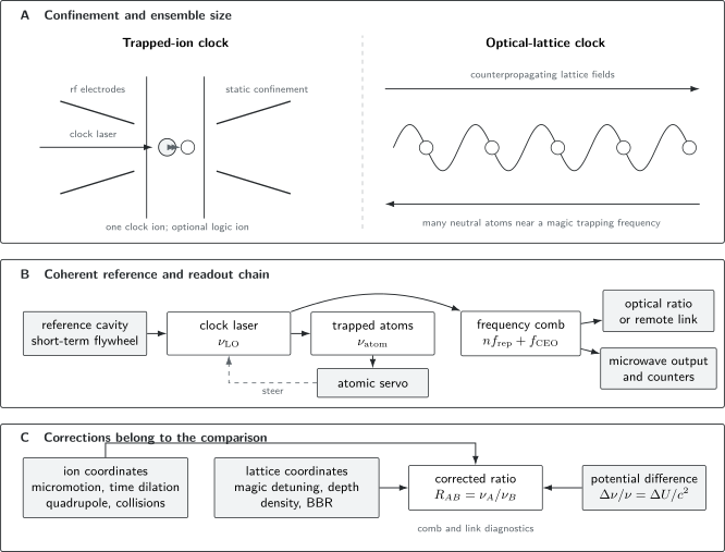
Modern optical clocks combine several logically distinct subsystems. A: a trapped-ion clock interrogates one or a few strongly confined particles, whereas a lattice clock interrogates many neutral atoms near the Lamb–Dicke regime at a magic trapping frequency. B: a cavity-stabilized laser is steered by atomic interrogation; a self-referenced frequency comb connects the optical output to another optical reference or to microwave electronics. C: ion and lattice clocks have different leading systematic coordinates, while every remote comparison also requires coherent transfer and a gravitational-potential correction.
One clock cycle
Section titled “One clock cycle”A representative cycle contains:
- Load and cool. Capture an ion or neutral-atom ensemble and reduce motion to the regime required by the uncertainty target.
- Prepare. Pump into a selected Zeeman or hyperfine clock state.
- Interrogate. Apply a phase-coherent Rabi, Ramsey, hyper-Ramsey, or related sequence with the clock laser.
- Detect. Infer the final state, often by electron shelving or state-dependent fluorescence.
- Discriminate. Probe opposite sides of the resonance, or use a phase-stepped sequence, to form an error signal.
- Steer. Update the laser frequency through an acousto-optic or electro-optic actuator.
- Evaluate. Interleave changed experimental conditions to estimate shifts and monitor auxiliary fields.
- Compare. Count a comb-derived beat, optical ratio, or coherent link observable with defined gates and signs.
The atoms need not be present continuously. During loading, cooling, and detection, the pre-stabilized laser carries the phase. The clock’s short-term stability can therefore be limited by local-oscillator noise and dead-time aliasing even when the atoms themselves are nearly ideal.
Optical Frequency References
Section titled “Optical Frequency References”Why optical frequencies help
Section titled “Why optical frequencies help”For uncorrelated atoms, a useful order-of-magnitude instability expression is
where is the coherent interrogation time, is fringe contrast, is the cycle time, and is the number of detected atoms per cycle. The exact numerical factor depends on the sequence, operating point, and detection model. The important optical-clock advantages are visible:
- large lowers the fractional error corresponding to a fixed phase error;
- narrow transitions permit long coherent interrogation;
- laser cooling and trapping suppress first-order Doppler broadening;
- carefully chosen clock states reduce sensitivity to fields; and
- frequency combs preserve phase while connecting optical and electronic frequencies.
The formula also exposes the platform trade-off. A single ion has but excellent isolation and readout. A lattice clock may interrogate to atoms, improving statistical precision, but must control collisions, inhomogeneity, and collective effects.
What makes a useful transition
Section titled “What makes a useful transition”A clock transition is judged as part of an instrument, not solely by its natural lifetime. Desirable properties include:
- a long-lived upper state and a linewidth narrower than the achievable interrogation linewidth;
- a wavelength for which coherent lasers and optical components are available;
- cooling, trapping, state-preparation, and detection transitions that can be operated reproducibly;
- clock states with small or characterizable differential electric and magnetic response;
- suppression of first-order Zeeman and electric-quadrupole shifts by angular-momentum choice or averaging;
- low sensitivity to blackbody radiation or accurately calculable polarizability;
- manageable motion, recoil, collisions, and probe shifts;
- independent clocks and ratio links for reproducibility; and
- atomic-structure sensitivity appropriate to any proposed fundamental-physics measurement.
The natural quality factor
can be enormous, but a finite pulse of duration produces a linewidth of order . The observed line can instead be limited by laser coherence, residual motion, magnetic noise, inhomogeneous shifts, or decoherence. Quoting as the achieved clock quality factor is therefore misleading unless lifetime-limited interrogation has actually been demonstrated.
Representative clock transitions
Section titled “Representative clock transitions”The following table gives rounded frequencies and wavelengths to identify important platforms. It is not a substitute for the isotope, hyperfine, Zeeman, polarization, and averaging conventions in a clock report.
| System | Representative clock transition | Frequency | Wavelength | Typical architecture |
|---|---|---|---|---|
| quantum-logic ion | ||||
| single ion | ||||
| electric-octupole line | single ion | |||
| electric-quadrupole line | single ion | |||
| single ion | ||||
| single ion | ||||
| optical lattice | ||||
| optical lattice | ||||
| optical lattice | ||||
| magnetically enabled | optical lattice |
Several of these radiations are secondary representations of the second in the BIPM list. That status means they can contribute to practical realizations and calibrations under specified procedures; it does not mean that each frequency is exact or that the SI second already has an optical definition.
Current SI status
Section titled “Current SI status”As of 25 July 2026, the SI second remains defined by assigning the exact value
to the unperturbed ground-state hyperfine transition of . Optical standards are measured against that definition directly or through an international least-squares network of absolute frequencies and optical ratios.
The CCTF approved an updated list of recommended standard frequencies in 2025, supported by published values and a covariance-aware adjustment. The BIPM roadmap discusses a possible redefinition in 2030 or later, conditional on agreed criteria for clock performance, independent reproducibility, frequency ratios, time and frequency transfer, operational reliability, and international access. A candidate transition, an ensemble of transitions, and the continuity strategy are matters of metrological decision, not consequences of a single laboratory record.
Narrow Optical Transitions
Section titled “Narrow Optical Transitions”Metastable states and forbidden lines
Section titled “Metastable states and forbidden lines”Strong electric-dipole transitions are excellent for cooling and fluorescence, but their short excited-state lifetimes make them too broad for the highest-resolution clocks. Clock lines are instead weak because a leading transition amplitude is forbidden or strongly suppressed by angular momentum, parity, spin, or multipole selection rules.
Examples include:
- intercombination transitions between and states in group-II-like atoms and ions;
- electric-quadrupole transitions such as ;
- an electric-octupole transition in ; and
- transitions made weakly allowed by hyperfine or magnetic mixing.
The same weak coupling that creates a narrow natural line makes coherent excitation technically demanding. Probe intensity, polarization, magnetic field, pulse area, phase noise, and off-resonant couplings must be known well enough that the interrogation itself does not dominate the clock.
Fermionic and bosonic lattice clocks
Section titled “Fermionic and bosonic lattice clocks”For fermionic isotopes such as and , hyperfine interaction mixes a small amount of character into the nominal state. The line is then weakly electric-dipole allowed. The nuclear spin also creates multiple Zeeman components. Clock operation usually prepares selected states and averages opposite projections to cancel the first-order Zeeman shift while retaining a magnetic-field diagnostic.
Even isotopes such as have nuclear spin zero. Their line lacks hyperfine-induced coupling and can be enabled by applying a static magnetic field that mixes the excited state with a nearby state. This offers simple level structure but introduces probe and magnetic-field dependencies that must be calibrated jointly.
These statements are architecture-level rules, not universal rankings. Fermions can suffer density-dependent -wave interactions and imperfect spin polarization; bosons can require larger enabling fields and can experience -wave collisions. The optimum isotope depends on atom number, geometry, temperature, interrogation protocol, and target uncertainty.
Clock laser and coherence
Section titled “Clock laser and coherence”During interrogation the local oscillator must preserve phase relative to the atomic superposition. A common chain is:
- lock a laser to a high-finesse reference cavity;
- suppress vibration, temperature, residual-amplitude, and optical-path noise;
- transfer that coherence to the atoms through a phase-stabilized path;
- steer the slowly varying laser frequency using the atomic error signal;
- compare or divide the disciplined light with a comb.
The cavity is a short-term flywheel. It does not provide the long-term accuracy of the clock transition. Thermal noise, drift, vibration, optical power, residual gas, and etalon effects move its resonance. Conversely, the atoms cannot correct laser phase between interrogations. Hybrid operation is essential.
For Rabi interrogation, the Fourier-limited line shape depends on pulse area and detuning. For Ramsey interrogation, the central-fringe scale is set mainly by the dark time. Rabi Oscillations and Ramsey Interferometry give the canonical derivations. Optical-clock reports should state the actual pulse duration, sequence, duty factor, contrast, atom number, and laser-noise conditions rather than infer them from the natural lifetime.
Probe-induced shifts
Section titled “Probe-induced shifts”Weak clock lines can require non-negligible probe intensity. Off-resonant coupling then produces an AC Stark shift. A sequence may reduce sensitivity by extrapolating to zero intensity, alternating intensities, using hyper-Ramsey phases, or adding a calibrated frequency step during the pulses.
Composite interrogation does not make the shift disappear automatically. Its cancellation relies on pulse area, phase, decoherence, frequency-step calibration, and servo symmetry. A valid evaluation varies those coordinates and tests the residual with an out-of-loop comparison.
Trapped Ions and Optical Lattices
Section titled “Trapped Ions and Optical Lattices”Single-ion clocks
Section titled “Single-ion clocks”A radio-frequency Paul trap or static-field Penning trap can confine an ion for long periods. Laser cooling places its secular motion near the Lamb–Dicke regime, so first-order Doppler broadening is suppressed. Strong cycling transitions provide nearly unit-efficiency state detection through electron shelving.
A representative single-ion sequence is:
- Doppler cool and, when required, sideband cool;
- optically pump into a clock-state Zeeman sublevel;
- turn off or control perturbing cooling light;
- interrogate the clock transition;
- detect whether fluorescence is bright or dark;
- repump and repeat at the opposite discriminator point.
The single particle avoids density shifts and makes state control clean. Its statistical limitation is also clear: one binary outcome is obtained per cycle. Improved laser coherence, longer interrogation, rapid cooling, high duty factor, and correlation with another clock can reduce the averaging time.
Quantum-logic clocks
Section titled “Quantum-logic clocks”Some excellent clock ions lack a convenient cycling transition. In quantum-logic spectroscopy, the clock ion is co-trapped with a logic ion. Shared motional modes provide a bus:
- the logic ion sympathetically cools the pair;
- the clock laser maps clock-state information to shared motion;
- logic operations map that motion to the logic ion;
- fluorescence of the logic ion reads out the clock state.
The canonical example is with a co-trapped logic ion. This architecture separates the species best suited to the reference transition from the species best suited to cooling and detection. It adds mode-frequency drift, heating, state-mapping fidelity, differential motion, collisions, and logic-pulse errors to the validation problem.
Quantum logic is not merely an indirect fluorescence detector. The mapping sequence and shared motion are part of the clock measurement model. A reported uncertainty must show that state-dependent mapping error does not move the lock point.
Ion-clock systematic coordinates
Section titled “Ion-clock systematic coordinates”Important ion-specific effects include:
- excess micromotion: displacement from the radio-frequency null creates driven motion and both time-dilation and rf Stark shifts;
- secular-motion time dilation: residual thermal and driven motion gives a relativistic second-order Doppler shift;
- electric-quadrupole shift: a state with nonzero quadrupole moment couples to static electric-field gradients;
- trap-induced AC Zeeman shift: rf currents and fields can perturb magnetic sublevels;
- background-gas collisions: rare events may shift phase, reorder an ion pair, or eject the ion;
- heating and mode drift: motion can change between cooling and interrogation; and
- logic-ion perturbations: cooling light, motion, and state-mapping operations can affect the clock ion.
For nonrelativistic speed , the time-dilation contribution is
The relevant includes secular motion, intrinsic micromotion, and excess micromotion under a stated model. It cannot be replaced by the Doppler-cooling temperature alone.
An electric-quadrupole shift has the angular structure
where is the state quadrupole moment, relates the quantization axis to a principal gradient axis, and represents the relevant traceless field-gradient component. Exact prefactors depend on tensor and gradient conventions. Averaging suitable Zeeman components or three orthogonal quantization axes can cancel a static rank-2 contribution, provided field directions, gradients, and weighting remain controlled.
Neutral-atom lattice clocks
Section titled “Neutral-atom lattice clocks”Neutral atoms cannot be confined as strongly by static electric fields. An optical lattice instead supplies a standing-wave AC Stark potential. Atoms are cooled and loaded into many lattice sites, where confinement suppresses recoil and first-order Doppler effects. Hundreds or thousands of atoms can be interrogated simultaneously.
The central design condition is that the ground and excited clock states experience equal leading-order light shifts. For lattice angular frequency , the electric-dipole magic condition is
At the magic frequency , the leading scalar E1 differential shift vanishes. The lattice still traps both states because their common polarizability need not vanish.
Magic operation does not imply zero lattice uncertainty. Residual terms can come from:
- detuning from the operational magic frequency;
- hyperpolarizability, proportional to higher powers of intensity;
- electric-quadrupole and magnetic-dipole lattice couplings;
- vector and tensor polarizabilities;
- imperfect polarization and magnetic-field alignment;
- motional-state dependence and tunneling;
- intensity inhomogeneity and longitudinal or transverse temperature;
- multiphoton or near-resonant structure; and
- correlations among fitted lattice-shift coefficients.
With the convention
a schematic differential shift is
Here denotes a convention-dependent differential hyperpolarizability, collects multipolar terms, and collects motion-dependent corrections. The numerical coefficients change if intensity or rms electric field is used instead of peak field. A clock paper must define the convention rather than transport coefficients blindly.
Collisions and many-body effects
Section titled “Collisions and many-body effects”Large atom number improves stability but introduces interactions. The observed shift can depend on:
- site occupancy and density;
- spin polarization and isotope statistics;
- excitation fraction;
- temperature and motional-state population;
- tunneling and lattice dimensionality;
- inhomogeneous Rabi coupling; and
- the interrogation sequence.
For identical spin-polarized fermions, -wave collisions are suppressed, but imperfect indistinguishability and -wave interactions remain. Bosonic isotopes permit -wave interactions. A common evaluation interleaves high and low atom number and fits a density coefficient, but a single linear slope is insufficient if excitation fraction or temperature co-varies with atom number.
Three-dimensional lattices can isolate atoms site by site and suppress collisions, at the cost of added lattice fields and more complex loading. One-dimensional lattices offer simpler optical geometry and high atom number, but may require stronger density and interaction controls.
Platform comparison
Section titled “Platform comparison”| Coordinate | Trapped-ion clock | Optical-lattice clock |
|---|---|---|
| Particle number | usually one clock ion | typically many neutral atoms |
| Statistical strength | one high-fidelity binary result per cycle | ensemble signal and fast averaging |
| Confinement | electromagnetic ion trap | state-insensitive optical lattice |
| Density shift | absent for a single clock ion | requires interaction evaluation |
| Motion | secular motion and micromotion | band, tunneling, temperature, recoil |
| Trap-light shift | usually no lattice field | magic condition plus residual lattice terms |
| Important tensor shift | electric quadrupole for suitable states | vector/tensor lattice and Zeeman terms |
| Readout | electron shelving; sometimes quantum logic | state-selective population detection |
| Duty factor | cooling and readout can be substantial | loading losses and destructive readout can be substantial |
| Strength | clean control and low interactions | high atom number and rapid stability |
| Main scaling challenge | single-particle statistics and trap fields | interactions, inhomogeneity, and lattice model |
No column is intrinsically more accurate. Uncertainty belongs to an evaluated realization under specified operating conditions. A clock with more favorable atomic coefficients can still perform worse if its fields, temperature, motion, or comparisons are inadequately controlled.
Stability and correlated interrogation
Section titled “Stability and correlated interrogation”For independent clocks, local-oscillator noise can dominate a comparison. Several strategies reduce it:
- increase laser coherence and interrogation duty factor;
- interrogate two ensembles synchronously with a common laser;
- use a second ensemble to estimate laser phase;
- operate zero-dead-time interleaved ensembles;
- transfer stability from a remote cryogenic or ultralow-noise cavity; or
- use entanglement or spin squeezing while accounting for loss and decoherence.
Synchronous comparison rejects laser noise only to the extent that the two systems share the same optical phase and sensitivity function. Differential path noise, unmatched pulse timing, unequal transfer functions, cycle slips, and asynchronous dead time reintroduce noise. Common-mode rejection can also hide a shared systematic, so absolute evaluations and independent links remain necessary.
Frequency-Comb Readout
Section titled “Frequency-Comb Readout”Signed comb equation
Section titled “Signed comb equation”A self-referenced comb has teeth
Let the clock laser beat with tooth at a signed beat frequency , and let acousto-optic modulators contribute signed shifts . One explicit convention is
The sign is determined by the physical optical-frequency ordering and diffraction path, not by whether a counter displays a positive number. A complete frequency record stores:
- the integer tooth index ;
- the definitions and signs of all beat notes;
- every fixed and time-dependent frequency shift;
- counter mode and gate timing;
- the comb locks and reference chain;
- cycle-slip diagnostics; and
- the optical reference plane to which the equation applies.
At , a one-tooth error is of order , often hundreds of megahertz. A sign error in a AOM is also enormous by clock standards. These are not small systematic corrections.
Absolute frequency and optical ratio
Section titled “Absolute frequency and optical ratio”An absolute frequency measurement expresses an optical transition in SI hertz. It must ultimately connect to the current caesium definition, usually through a microwave reference, a local time scale, satellite or fiber transfer, and primary or secondary standard calibrations. The comparison uncertainty and dead time can be much larger than the intrinsic optical-clock uncertainty.
An optical frequency ratio
can be measured directly with a comb while avoiding much of the microwave chain. Because a ratio of frequencies is dimensionless, it is also the natural observable for comparing atomic structure and searching for changes in dimensionless constants.
Direct ratios do not eliminate all conventions. Both frequencies need systematic and gravitational corrections to declared reference conditions. Comb transfer noise, uncompensated paths, counter synchronization, data selection, and covariance among clocks must be evaluated.
Transfer-oscillator principle
Section titled “Transfer-oscillator principle”Two lasers at and produce beat signals against teeth and . Suitable electronic or digital combinations can cancel comb fluctuations in and without requiring the comb itself to be quieter than either optical source. In schematic form, construct a transfer observable
with signs and AOM terms adapted to the actual optical layout. Substitution of the tooth equations removes the repetition-rate noise. The exact implementation must account for electronic delays, finite bandwidth, integer ratios, synthesizer phase noise, and sampled data timing.
Frequency Combs gives the full derivation. The operational lesson for clocks is that a comb is a coherent gearbox: it transfers a reference and its noise. It does not independently certify either clock.
Ratio closure
Section titled “Ratio closure”For three co-located, simultaneously defined frequencies,
A measured logarithmic closure residual is
Closure is a powerful check on comb signs, transfer chains, and ratio consistency. It is not a proof that all clocks are unbiased. A shared systematic shift can cancel from closure, and ratios measured at different times require a model for drift and covariance.
Remote optical comparisons
Section titled “Remote optical comparisons”Remote clocks can be compared through actively stabilized optical fiber, free-space optical time-frequency transfer, transportable clocks, or satellite-based methods. The comparison observable includes:
- the two local clock corrections;
- local comb and synthesis chains;
- link phase-noise cancellation and residual asymmetry;
- cycle-slip and data-validity monitors;
- synchronized counter gates or a model for asynchronous sampling; and
- the gravitational-potential difference between reference locations.
At the level, the optical path through a laboratory, a patch cord exposed to temperature, or an incorrectly defined endpoint can matter. The phrase “fiber link uncertainty” is incomplete unless the physical reference planes and both local branches are included.
Systematic Shift Architecture
Section titled “Systematic Shift Architecture”Measurement model
Section titled “Measurement model”Write the fractional observation model as
where is the target fractional frequency, are systematic shifts, and is statistical fluctuation under a specified averaging protocol. If the estimated corrections are collected in , then
For covariance matrix , the systematic variance of the sum is
Optical-clock coefficients are often shared across days, apparatuses, or species. Treating all entries as independent can understate or overstate uncertainty. The covariance model should distinguish measured environmental coordinates, fitted coefficients, atomic-theory inputs, and common calibrations.
Systematic ledger
Section titled “Systematic ledger”| Effect | Representative coordinate | Typical validation |
|---|---|---|
| Blackbody radiation | temperature field, static polarizability, dynamic correction | thermal map, sensor calibration, heated or cryogenic test |
| DC Stark | stray electric field, electrode charge | field reversal, compensation scan |
| Lattice Stark | depth, frequency, polarization, motional state | interleaved depth/frequency scan and model fit |
| Probe Stark | pulse intensity and timing | intensity extrapolation or composite-sequence test |
| Zeeman | field magnitude, direction, sublevel | opposite- averaging and field scan |
| Electric quadrupole | field gradient and quantization axis | sublevel or three-axis averaging |
| Time dilation | secular motion, micromotion, temperature | sideband thermometry and micromotion diagnostics |
| Collisions | density, excitation, background gas | density interleave, collision monitoring |
| Servo | discriminator asymmetry, drift, gain | modulation reversal and synthetic injection |
| Line pulling | neighboring transitions, unwanted populations | state purification and spectrum scan |
| Gravitational | geopotential at the atomic reference point | geodetic survey and potential model |
| Transfer chain | comb, AOM, fiber, counters | redundant beats, closure, synchronized gates |
A correction can be small while its uncertainty is large, and a large correction can be known accurately. Ranking effects only by correction magnitude is therefore unsound.
Blackbody and Stark Shifts
Section titled “Blackbody and Stark Shifts”Blackbody radiation
Section titled “Blackbody radiation”Thermal electromagnetic radiation produces a differential AC Stark shift. For an approximately isotropic environment at temperature , a common parameterization is
where is the differential static polarizability, is a dynamic correction, and
The proportionality is exact for an ideal blackbody field when expressed through the radiation energy density; apertures, emissivity, view factors, temperature gradients, and non-equilibrium surfaces make the apparatus model more complicated.
If the term dominates and coefficient uncertainty is neglected, then
This derivative is useful for planning but not a complete BBR budget. One must also propagate uncertainties in polarizability, dynamic correction, effective radiation temperature, gradients, emissivity, and the atom’s view of hot ovens, windows, electrodes, or apertures.
Three broad strategies are used:
- operate near room temperature and measure the full thermal environment;
- surround the atoms with a well-characterized radiation shield; or
- operate cryogenically to reduce both the shift and its temperature sensitivity.
Temperature sensors report their own locations. The atoms sample a radiative field assembled from all visible surfaces. The two quantities coincide only under a validated thermal and radiative model.
DC electric fields
Section titled “DC electric fields”A static field produces, to leading scalar order,
Patch charge on dielectrics, ultraviolet illumination, electrode contamination, and photoemission can create slowly varying fields. Because the leading shift is quadratic, simply reversing one electrode voltage does not necessarily reverse the shift. A compensation scan in several directions, together with a field model, is more informative.
Lattice Stark model
Section titled “Lattice Stark model”Near the magic frequency, expand the differential E1 polarizability:
The leading residual shift is therefore bilinear in lattice intensity and magic-frequency detuning. At high depth, hyperpolarizability and multipolar terms can be comparable to the target uncertainty. An operational magic condition may deliberately choose a detuning and depth where several terms have reduced first derivative, rather than identifying one universal zero independent of motional state and intensity.
A robust evaluation samples a grid of depths and frequencies, not only two depths at one nominal wavelength. It records polarization, atom temperature, axial and radial occupation, and correlations among fitted coefficients. Extrapolating a polynomial outside the measured operating region is especially hazardous.
Magnetic shifts
Section titled “Magnetic shifts”For a clock component labeled by , a schematic expansion is
Averaging symmetric components gives
while their difference monitors the field:
This cancellation assumes the two components sample the same field, interrogation, and time. Magnetic drift between sequential probes, unequal line pulling, polarization error, tensor shifts, and servo weighting can leave a residual. The quadratic shift remains and must be measured or calculated.
Motion and recoil
Section titled “Motion and recoil”The Lamb–Dicke regime suppresses first-order Doppler effects because the particle explores a region small compared with the probe wavelength. It does not eliminate:
- relativistic time dilation;
- recoil and motional-state dependence;
- phase shifts from wave-front curvature or beam misalignment;
- micromotion in an rf ion trap;
- lattice tunneling and band effects; or
- Doppler shifts from uncompensated optical-path motion.
For an optical phase delivered along path length , mirror or fiber motion changes the phase at the atoms. Active path stabilization must sense the relevant endpoint. Stabilizing to a nearby mirror while leaving a moving segment between that mirror and the atoms can produce an interrogation-synchronous frequency error.
Collisions and background gas
Section titled “Collisions and background gas”Neutral-atom density shifts are usually measured by interleaving populations and fitting frequency versus a density proxy. The proxy itself may depend on detection gain, cloud size, excitation fraction, temperature, and site occupancy. A trustworthy evaluation:
- defines the density observable;
- randomizes or balances the interleave order;
- checks linearity and excitation dependence;
- propagates uncertainty in the extrapolation point; and
- tests for correlations with lattice depth and loading.
Single-ion clocks avoid clock-ion density shifts but not background-gas collisions. Collision-induced phase steps can have non-Gaussian distributions, and energetic collisions can change the ion crystal without immediate loss. Event cuts require predeclared diagnostics and a bias test.
Servo and line-shape errors
Section titled “Servo and line-shape errors”A clock servo can be biased by:
- unequal sampling of the two line slopes;
- cavity or laser drift during the modulation sequence;
- different atom number or contrast at alternate points;
- line-shape asymmetry and neighboring transitions;
- digital quantization, saturation, or integrator leakage;
- feed-forward error;
- imperfect frequency steps during composite pulses; and
- data rejection correlated with the measured detuning.
Useful tests include reversing probe order, changing servo gain and update law, injecting a known synthetic offset, locking with independent discriminators, and comparing against another clock. Agreement of an in-loop error signal with zero is expected for a working servo and is not an independent validation.
Clock Comparisons and Accuracy
Section titled “Clock Comparisons and Accuracy”Stability is not uncertainty
Section titled “Stability is not uncertainty”A typical optical-clock comparison may average approximately as
over a range of . This describes a noise process under the stated measurement conditions. It does not show that the mean is unbiased or that the uncertainty budget is complete.
Conversely, a systematic uncertainty of is not a noise floor that every Allan-deviation curve must reach. A constant unknown offset does not contribute to Allan deviation, and correlated drift may average differently from white frequency noise. Reports should show stability analysis, corrected means, systematic ledgers, and comparison statistics separately.
Independent reproducibility
Section titled “Independent reproducibility”The strongest evidence for an optical standard combines:
- repeated evaluations over changed conditions and long times;
- two clocks of the same species with substantially independent apparatus;
- ratios between different species;
- redundant combs or transfer chains;
- remote comparisons through independently characterized links;
- closure tests across a network;
- blinded or precommitted analysis where feasible; and
- uncertainty normalized residuals across laboratories.
Same-species agreement is sensitive to differential implementation errors but can miss shared atomic-theory or environmental assumptions. Different-species ratios probe different sensitivities but add a second clock’s systematic ledger. A mature evidence program uses both.
Date-stamped performance examples
Section titled “Date-stamped performance examples”Performance numbers are moving targets and should always carry dates and conditions. Examples that illustrate architecture rather than establish a permanent ranking include:
- optical lattice clocks have demonstrated total systematic uncertainties in the low- range and below;
- a 2025 quantum-logic clock reported systematic uncertainty and instability using a one-second Rabi probe and remotely transferred laser stability; and
- a three-species optical network reported Al/Yb, Al/Sr, and Yb/Sr ratios with fractional uncertainties at or below in 2021.
These results are not interchangeable. A systematic uncertainty, a comparison uncertainty, and a one-second instability answer different questions. They also depend on the reported coverage convention, correlations, data selection, and reference conditions.
Relativistic Geodesy
Section titled “Relativistic Geodesy”Clocks measure gravitational potential
Section titled “Clocks measure gravitational potential”In the weak-field, slow-motion limit, two stationary clocks at gravitational potentials differing by have
Near Earth’s surface, for a small vertical displacement in an approximately uniform field,
The sign depends on the definition of and which clock is in the numerator. With the usual convention, a clock at higher gravitational potential runs faster.
The centimeter conversion is a local approximation. A clock measures potential, not geometric height alone. Precise work includes:
- Earth’s gravitational potential and its temporal variation;
- centrifugal potential in the rotating terrestrial frame;
- solid-Earth and ocean tides;
- atmospheric and hydrological mass redistribution;
- the reference potential used for conventional relativistic corrections;
- coordinates of the atomic reference point; and
- the potential difference along the comparison epoch.
Geodetic leveling and gravimetry remain necessary to interpret or validate the clock result. Optical clocks add a direct potential-difference observable and can connect separated height systems, monitor changes, or test geopotential models.
Local and remote clock geodesy
Section titled “Local and remote clock geodesy”A local vertical comparison may use two clocks in one building connected by phase-stabilized fiber. A remote comparison can use:
- fixed optical clocks linked through a fiber network;
- a transportable clock brought to the field site;
- free-space optical transfer;
- a clock network tied through an intermediate transfer laser; or
- hybrid optical and satellite techniques.
For corrected ratio , a schematic measurement model is
is the ratio for a declared common reference potential. The link and both clock corrections must be estimated before interpreting the residual as geopotential.
What geodesy claims require
Section titled “What geodesy claims require”A defensible clock-geodesy result states:
- which atomic reference points and epochs define the comparison;
- the frequency-ratio sign and gravitational-potential convention;
- the geodetic datum or reference potential;
- the clock, link, and geodetic uncertainty components and covariance;
- tidal and loading corrections;
- how transport, restart, or relocation shifts were tested; and
- whether the result estimates potential, geopotential number, or an equivalent height under a specified gravity model.
“The clock measured height” is shorthand only after these choices are declared.
Fundamental Tests
Section titled “Fundamental Tests”Frequency ratios and dimensionless constants
Section titled “Frequency ratios and dimensionless constants”Atomic transition frequencies depend differently on dimensionless constants because relativistic, hyperfine, nuclear, and many-electron contributions differ. For a ratio , a linearized model is
Here is the fine-structure constant and, on this page,
Some literature defines , which reverses the associated sensitivity coefficient. Every analysis must state the convention.
The coefficients come from atomic, molecular, and nuclear-structure calculations. A measured ratio drift constrains a combination of parameters. It becomes a bound on one constant only after assuming the others are fixed or combining enough independent observables to estimate them.
Local position invariance
Section titled “Local position invariance”A phenomenological redshift-violation model can assign each clock species a parameter :
General relativity predicts . A co-located ratio measured while the laboratory potential changes is sensitive to , not to a common universal term. Annual solar-potential modulation, terrestrial height comparisons, and spacecraft or tower experiments test different combinations of assumptions and systematics.
Environmental annual cycles can mimic a potential-correlated signal. Temperature, magnetic fields, humidity, electronics, link behavior, and data availability must be included in the nuisance model. Choosing the phase or period after inspecting the data also changes the statistical interpretation.
Oscillatory and transient searches
Section titled “Oscillatory and transient searches”Some ultralight dark-matter models predict coherent oscillations of effective constants and therefore of clock ratios. A representative template is
where depends on a specified field density, coupling model, and sensitivity coefficients. Networks can also search for transient, correlated disturbances.
A null clock residual is not a model-independent exclusion of dark matter. A valid limit requires:
- a Lagrangian or explicit coupling parameterization;
- assumptions about field density, coherence time, and velocity distribution;
- clock response and sampling transfer functions;
- calibrated timing and network geometry;
- treatment of gaps, colored noise, and systematics;
- trials factors for a frequency or event-time scan; and
- a declared confidence or credible-interval construction.
Clock networks can be exceptionally sensitive within such models because ratios are precise and geographically separated instruments provide correlation tests. The interpretation remains conditional.
Lorentz and other symmetry tests
Section titled “Lorentz and other symmetry tests”Clock transitions can test Lorentz symmetry by searching for orientation- or boost-dependent frequency changes as Earth rotates and orbits. The observable may involve Zeeman sublevels with anisotropic electronic momentum sensitivity rather than the field-insensitive component optimized for timekeeping. Magnetic fields, tensor Stark shifts, quadrupole shifts, laboratory orientation, and sidereal-versus-solar aliases become central.
The result constrains coefficients in a specified effective theory and frame convention. It should not be summarized as a universal “test of Lorentz invariance” without naming the sector and coefficient combination.
Building a Trustworthy Optical-Clock Result
Section titled “Building a Trustworthy Optical-Clock Result”Reproducible workflow
Section titled “Reproducible workflow”A mature optical-clock campaign should preserve enough information to reconstruct the result:
- Define the measurand. State isotope, transition, Zeeman or hyperfine averaging, rest-frame convention, reference potential, and epoch.
- Freeze sign conventions. Document comb beats, AOM shifts, ratio order, correction signs, and relativistic potential signs.
- Record raw cycle data. Preserve excitation, atom number, servo state, environmental monitors, validity flags, and timing.
- Calibrate transfer functions. Measure discriminator slope, servo response, optical-path response, and counter behavior.
- Interleave systematics. Randomize or balance changed conditions and preserve the complete sequence.
- Propagate covariance. Keep common coefficients and calibrations correlated across days and clocks.
- Blind high-impact choices. Where practical, hide the final ratio or inject a secret offset while cuts and models are settled.
- Compare independently. Use another clock, comb, link, species, or analysis path.
- Audit residuals. Examine dependence on time, operating coordinates, data quality, and environmental variables.
- Publish evidence. Report enough metadata, code, covariance, and corrected data for an informed reanalysis.
Common mistakes
Section titled “Common mistakes”Calling the atom the clock
Section titled “Calling the atom the clock”The atomic transition is the reference. The running output comes from a laser, servo, synthesis chain, and counter. Noise or bias in any of them can move the delivered frequency.
Equating a narrow line with accuracy
Section titled “Equating a narrow line with accuracy”Linewidth determines resolution and potential stability. Accuracy requires an evaluated shift model and comparison evidence.
Treating the magic wavelength as exact and universal
Section titled “Treating the magic wavelength as exact and universal”The operational zero can depend on lattice depth, polarization, motional state, hyperpolarizability, multipolar terms, and fit convention.
Assuming symmetric-state averaging cancels everything
Section titled “Assuming symmetric-state averaging cancels everything”Opposite Zeeman states cancel the leading odd-in- term under matched sampling. Quadratic Zeeman, tensor Stark, drift, line pulling, and unequal weights remain.
Using room temperature instead of radiation temperature
Section titled “Using room temperature instead of radiation temperature”A sensor value is not automatically the effective temperature seen by the atoms. View factors, gradients, windows, ovens, and emissivity matter.
Dropping AOM and beat-note signs
Section titled “Dropping AOM and beat-note signs”Counters display magnitudes. Frequency equations require signed optical ordering and every pass through every modulator.
Calling an optical ratio an absolute frequency
Section titled “Calling an optical ratio an absolute frequency”A ratio is dimensionless and can avoid the microwave chain. An absolute frequency in SI hertz must connect to the caesium-defined second.
Ignoring gravitational potential
Section titled “Ignoring gravitational potential”Two accurate clocks at different potentials should disagree before the relativistic correction. At , centimeters matter.
Reading a model-independent discovery into a ratio residual
Section titled “Reading a model-independent discovery into a ratio residual”Variation-of-constants, redshift-violation, dark-matter, and Lorentz tests depend on sensitivity coefficients, effective-theory conventions, environmental models, and statistical trials.
Further Connections
Section titled “Further Connections”- Atomic Clocks for Quantum Estimation develops oscillator tracking, information rate, phase slips, entangled probes, synchronous comparisons, and evidence for a running-clock quantum gain.
- Ramsey Interferometry for Quantum Estimation develops the fringe likelihood, local and global identifiability, interrogation-time optimization, and wall-clock information rate.
- Spin Squeezing develops collective-state preparation, Wineland gain, entanglement certification, and the distinction between state-level and running-clock improvements.
- Distributed Quantum Sensing develops remote-clock difference estimators, inter-node entanglement benchmarks, synchronization, reference-frame, and information-rate costs.
- Optical Clock Frontiers
- Precision Measurement and Metrology
- Atomic Clocks
- Frequency Standards
- Variation of Constants Searches
- Precision Spectroscopy
- Ramsey Interferometry
- Rabi Oscillations
- Frequency Combs
- Laser Stabilization
- Ion Traps
- Optical Lattices
- AC Stark Shift
- Dynamic Polarizability
- Zeeman Effect in Atoms
- Hyperfine Structure
- Quantum Sensing
References
Section titled “References”- Bureau International des Poids et Mesures, The International System of Units (SI Brochure), 9th ed., version 4.01 (June 2026), doi:10.59161/AUEZ1291.
- Bureau International des Poids et Mesures, “Recommended values of standard frequencies: for the second,” updated following the 2025 adjustment, BIPM standard-frequency list.
- H. S. Margolis et al., “Data associated with the 2025 adjustment of standard frequencies” (2026), doi:10.59161/StdFreq2026.
- Bureau International des Poids et Mesures, “Roadmap to the redefinition of the second,” updated March 2025, BIPM redefinition portal.
- N. Dimarcq et al., “Roadmap towards the redefinition of the second,” Metrologia 61, 012001 (2024), doi:10.1088/1681-7575/ad17d2.
- T. M. Fortier, A. N. Luiten, and H. S. Margolis, “Optical atomic clocks: defining the future of time and frequency metrology,” Optica 13, 143–163 (2026), doi:10.1364/OPTICA.575770.
- A. D. Ludlow, M. M. Boyd, J. Ye, E. Peik, and P. O. Schmidt, “Optical atomic clocks,” Reviews of Modern Physics 87, 637–701 (2015), doi:10.1103/RevModPhys.87.637.
- H. Katori, M. Takamoto, V. G. Pal’chikov, and V. D. Ovsiannikov, “Ultrastable optical clock with neutral atoms in an engineered light shift trap,” Physical Review Letters 91, 173005 (2003), doi:10.1103/PhysRevLett.91.173005.
- A. Derevianko and H. Katori, “Colloquium: Physics of optical lattice clocks,” Reviews of Modern Physics 83, 331–347 (2011), doi:10.1103/RevModPhys.83.331.
- P. O. Schmidt et al., “Spectroscopy using quantum logic,” Science 309, 749–752 (2005), doi:10.1126/science.1114375.
- S. M. Brewer et al., “ quantum-logic clock with a systematic uncertainty below ,” Physical Review Letters 123, 033201 (2019), doi:10.1103/PhysRevLett.123.033201.
- M. C. Marshall et al., “High-stability single-ion clock with systematic uncertainty,” Physical Review Letters 135, 033201 (2025), doi:10.1103/hb3c-dk28.
- T. L. Nicholson et al., “Systematic evaluation of an atomic clock at total uncertainty,” Nature Communications 6, 6896 (2015), doi:10.1038/ncomms7896.
- W. F. McGrew et al., “Atomic clock performance enabling geodesy below the centimetre level,” Nature 564, 87–90 (2018), doi:10.1038/s41586-018-0738-2.
- E. Oelker et al., “Demonstration of stability at for two independent optical clocks,” Nature Photonics 13, 714–719 (2019), doi:10.1038/s41566-019-0493-4.
- T. Bothwell et al., “Resolving the gravitational redshift across a millimetre-scale atomic sample,” Nature 602, 420–424 (2022), doi:10.1038/s41586-021-04349-7.
- M. Takamoto et al., “Test of general relativity by a pair of transportable optical lattice clocks,” Nature Photonics 14, 411–415 (2020), doi:10.1038/s41566-020-0619-8.
- J. Grotti et al., “Geodesy and metrology with a transportable optical clock,” Nature Physics 14, 437–441 (2018), doi:10.1038/s41567-017-0042-3.
- C. Lisdat et al., “A clock network for geodesy and fundamental science,” Nature Communications 7, 12443 (2016), doi:10.1038/ncomms12443.
- Boulder Atomic Clock Optical Network Collaboration, “Frequency ratio measurements at 18-digit accuracy using an optical clock network,” Nature 591, 564–569 (2021), doi:10.1038/s41586-021-03253-4.
- S. M. Middelmann, C. Lisdat, S. Falke, J. S. R. Vellore Winfred, F. Riehle, and U. Sterr, “Tackling the blackbody shift in a strontium optical lattice clock,” IEEE Transactions on Instrumentation and Measurement 60, 2550–2557 (2011), doi:10.1109/TIM.2010.2088470.
- S. G. Porsev and A. Derevianko, “Multipolar theory of blackbody radiation shift of atomic energy levels and its implications for optical lattice clocks,” Physical Review A 74, 020502(R) (2006), doi:10.1103/PhysRevA.74.020502.
- R. C. Brown et al., “Hyperpolarizability and operational magic wavelength in an optical lattice clock,” Physical Review Letters 119, 253001 (2017), doi:10.1103/PhysRevLett.119.253001.
- M. Bishof et al., “Inelastic collisions and density-dependent excitation suppression in a optical lattice clock,” Physical Review A 84, 052716 (2011), doi:10.1103/PhysRevA.84.052716.
- T. Rosenband et al., “Frequency ratio of Al and Hg single-ion optical clocks; metrology at the 17th decimal place,” Science 319, 1808–1812 (2008), doi:10.1126/science.1154622.
- M. S. Safronova et al., “Search for new physics with atoms and molecules,” Reviews of Modern Physics 90, 025008 (2018), doi:10.1103/RevModPhys.90.025008.
- N. Huntemann, B. Lipphardt, C. Tamm, V. Gerginov, S. Weyers, and E. Peik, “Improved limit on a temporal variation of from comparisons of Yb and Cs atomic clocks,” Physical Review Letters 113, 210802 (2014), doi:10.1103/PhysRevLett.113.210802.
- F. Riehle, “Optical clock networks,” Nature Photonics 11, 25–31 (2017), doi:10.1038/nphoton.2016.235.
- T. Mehlstäubler, G. Grosche, C. Lisdat, P. O. Schmidt, and H. Denker, “Atomic clocks for geodesy,” Reports on Progress in Physics 81, 064401 (2018), doi:10.1088/1361-6633/aab409.
- C. Sanner et al., “Optical clock comparison for Lorentz symmetry testing,” Nature 567, 204–208 (2019), doi:10.1038/s41586-019-0972-2.
- M. Filzinger et al., “Improved limits on the coupling of ultralight bosonic dark matter to photons from optical atomic clock comparisons,” Physical Review Letters 130, 253001 (2023), doi:10.1103/PhysRevLett.130.253001.
Exercises
Section titled “Exercises”1. Optical quality factor and interrogation
Section titled “1. Optical quality factor and interrogation”A strontium lattice clock operates at and uses a one-second Rabi pulse. For an estimate, take the interrogation-limited linewidth to be .
- Estimate the linewidth.
- Find the corresponding observed quality factor.
- A metastable lifetime would imply a natural linewidth of . Find the natural quality factor.
- Explain which quality factor should be used to describe the observed discriminator.
Solution
With ,
The observed quality factor is
For a natural linewidth of ,
The observed discriminator is set by the actual pulse, laser coherence, contrast, and decoherence, so is the relevant realized value. describes the transition’s lifetime-limited potential and should not be presented as the measured linewidth.
2. A signed comb measurement
Section titled “2. A signed comb measurement”A clock laser is above comb tooth . The comb has
The positive beat magnitude is . The light then passes once through a AOM before reaching the atoms.
- Write the signed frequency equation at the atoms.
- Calculate the optical frequency.
- Find the error caused by using the wrong beat-note sign.
- Find the error caused by forgetting the AOM.
Solution
“Above the tooth” gives , and the AOM is explicitly a positive shift:
The tooth contribution is
Therefore
Changing to changes the answer by . Forgetting the AOM changes it by . Both errors are vastly larger than any optical-clock uncertainty.
3. Residual lattice shift near the magic frequency
Section titled “3. Residual lattice shift near the magic frequency”Near an operational point, suppose the measured fractional lattice shift is modeled by
where is in megahertz and is the trap depth in units of . Let
Evaluate the shift at and . Then find the frequency detuning that makes this two-term model zero at the same depth.
Solution
At the stated point,
For zero shift at fixed ,
Thus
The result illustrates an operational magic point: cancellation at one depth need not identify the zero of the E1 polarizability alone.
4. Blackbody temperature uncertainty
Section titled “4. Blackbody temperature uncertainty”At , a clock has a fractional BBR correction of . Treat the shift as exactly proportional to and let the standard uncertainty of the effective radiation temperature be .
- Find the fractional uncertainty contributed by temperature.
- How small must be for this contribution to be ?
- Name three omitted contributions in a real BBR evaluation.
Solution
The relative sensitivity of the shift is
Therefore
For a target of ,
Thus the effective radiation temperature would need a standard uncertainty of about under this simplified model. Real evaluations also include differential polarizability, dynamic correction, gradients, view factors, surface emissivities, hot apertures, and sensor calibration and self-heating.
5. Ion time dilation
Section titled “5. Ion time dilation”An ion’s total rms speed during interrogation is estimated as .
- Find the fractional time-dilation shift.
- Find the absolute shift of a transition.
- Why can the result not be assigned solely to the secular temperature without further evidence?
Solution
Using ,
The absolute shift is
The velocity variance can include secular motion, intrinsic micromotion, excess micromotion, driven motion, and heating during the dark interval. A secular temperature alone does not determine all of these components.
6. A gravitational-potential comparison
Section titled “6. A gravitational-potential comparison”Clock is above clock in a laboratory where . Ignore tides and use a uniform field.
- Find .
- If the measured corrected ratio residual is , is it consistent with the height model at one standard uncertainty?
- What equivalent height corresponds to a fractional uncertainty of ?
Solution
The potential difference is
Hence
The residual difference from the model is
This is times the stated standard uncertainty , so it is consistent at one standard uncertainty.
The equivalent local height uncertainty is
Thus the simplified conversion is about . A real result is an uncertainty in potential; conversion to height requires a gravity and geodetic model.
7. Sensitivity to variation of the fine-structure constant
Section titled “7. Sensitivity to variation of the fine-structure constant”Two clock transitions have and . Suppose their measured ratio drift is
Assume for this exercise that only varies.
- Infer and its standard uncertainty.
- Explain why this is not a model-independent statement about all constants.
- If an unmodeled annual temperature systematic exists, what additional evidence would be useful?
Solution
Under the one-parameter assumption,
Therefore
The inference assumes other dimensionless parameters are constant and the sensitivity coefficients are correct. More general models require additional independent clock and molecular ratios to separate parameter combinations.
Useful evidence includes measured temperature sensitivities, environmental regression fixed before looking at the final drift, multiple years of data, comparison with another laboratory and climate, residual spectra, and ratios with different . An annual signal alone can alias solar potential, temperature, humidity, and data-availability cycles.
8. Design and audit an optical-clock comparison
Section titled “8. Design and audit an optical-clock comparison”Design one of the following:
- a local Al/Yb optical ratio;
- a remote Sr/Sr relativistic-geodesy comparison;
- a transportable Sr clock campaign;
- a Yb/Sr test of constant variation; or
- a same-species comparison of two independent lattice clocks.
Specify:
- the measurand and ratio orientation;
- clock transition and interrogation for each endpoint;
- clock-laser and comb architecture;
- at least six platform-specific systematic effects per clock;
- path, link, and counter diagnostics;
- gravitational-potential treatment;
- covariance and data-selection model;
- at least three reversal or interleaving tests; and
- the evidence that would distinguish a clock discrepancy from a link or analysis discrepancy.
Solution
There is no unique solution. For a remote Sr/Sr geodesy comparison, a defensible design uses two independently evaluated lattice clocks and defines
at a common conventional reference potential. Each laboratory operates a cavity-prestabilized clock laser, symmetric averaging, phase-stable delivery to the atoms, and an atomic servo. A coherent telecom transfer laser and self-referenced comb at each endpoint bridge the clock wavelength to a bidirectionally stabilized fiber.
Each clock ledger includes BBR, lattice E1 detuning, hyperpolarizability, multipolar and motional lattice shifts, quadratic Zeeman shift, density shift, probe shift, line pulling, optical-path phase, servo error, and background-gas collisions. The link ledger includes local uncompensated fibers, bidirectional asymmetry, interferometer offsets, amplifiers, cycle slips, comb transfer, AOM signs, counter dead time, and gate synchronization.
The geodetic model states both atomic reference points, comparison epochs, tidal and loading corrections, centrifugal potential, datum, and covariance between survey and gravity observations. Useful reversals include high/low lattice depth, high/low density, opposite Zeeman components, reversed probe order, alternate combs, and a deliberately changed link path.
To localize a discrepancy, preserve simultaneous local ratio beats, round-trip link diagnostics, independent comb channels, raw clock excitations, and common-view intervals. A transportable third clock or a loop with a second link can add closure. Agreement after swapping combs but not after bypassing a local fiber implicates the local transfer branch; agreement locally but not remotely implicates the link or geopotential model; disagreement between independently corrected local clocks implicates a clock ledger or shared optical reference. The conclusion must follow these diagnostics rather than the preferred application.