Dynamic Polarizability

The dynamic electric-dipole polarizability describes how a quantum state responds linearly to an electric field of angular frequency $\omega$. It is not generally a single material constant. It depends on the state, drive frequency, polarization, quantization geometry, and convention used for the complex field.

For a monochromatic field written with peak amplitude $E_0$,

$$\mathbf E(t) = \operatorname{Re} \left[ E_0\boldsymbol\epsilon e^{-i\omega t} \right], \qquad \boldsymbol\epsilon^* \mathbin{\cdot} \boldsymbol\epsilon = 1,$$

the induced dipole amplitude is

$$\mathbf d^{(+)} = \boldsymbol\alpha_a(\omega) \mathbin{\cdot} E_0\boldsymbol\epsilon.$$

The tensor $\boldsymbol\alpha_a(\omega)$ is complex when absorption, stimulated emission, ionization, or radiative loss is resolved. Its real part produces the leading conservative light shift, while its imaginary part encodes dissipative response:

$$U_a = - \frac{E_0^2}{4} \operatorname{Re} \left[ \boldsymbol\epsilon^* \mathbin{\cdot} \boldsymbol\alpha_a(\omega) \mathbin{\cdot} \boldsymbol\epsilon \right].$$

The central physical lesson is that polarizability is a spectral sum. Every dipole-coupled level contributes with a frequency denominator. Poles, zeros, signs, and state-insensitive trapping conditions arise from how those contributions reinforce or cancel.

Canonical Scope

This page owns the frequency-dependent response calculation:

1. the induced-dipole and linear-response definitions;
2. the causal tensor sum over discrete and continuum intermediate states;
3. the rotating and counter-rotating frequency denominators;
4. static, resonant, and high-frequency consistency checks;
5. real and imaginary response near broadened resonances;
6. scalar, vector, and tensor reduction for angular-momentum states;
7. tune-out zeros and magic crossings;
8. uncertainty-aware calculations for optical trapping and clocks.

Nearby pages have narrower responsibilities:

• AC Stark Shift owns the exact driven two-state quasienergies, far-detuned expansion, Bloch–Siegert correction, and shift–scattering tradeoff.
• Stark Effect in Atoms owns the atom-specific DC response, degeneracy structure, alkali examples, and spectroscopic interpretation.
• Linear Response Preview owns the general retarded-susceptibility and absorbed-power derivation.
• Second-Order Energy Corrections owns the stationary perturbation-theory structure behind the static limit.
• Optical Bloch Equations owns saturation, power broadening, and population dynamics when a resonant line cannot be treated as a weak linear response.
• Scalar, Vector, and Tensor Operators owns the general irreducible-tensor algebra.
• Precision Spectroscopy owns complete measurement protocols and systematic-uncertainty budgets.

Convention Ledger

The formulas below use:

• a field-free eigenstate $|a\rangle$ with energy $E_a$;

• intermediate eigenstates $|n\rangle$ with signed Bohr frequencies

  $$\omega_{na} = \frac{E_n-E_a}{\hbar};$$

• the electric-dipole operator $\mathbf d$;

• time dependence $e^{-i\omega t}$ for positive-frequency amplitudes;

• a complex unit polarization vector $\boldsymbol\epsilon$;

• peak electric amplitude $E_0$, not an RMS amplitude;

• vacuum intensity

  $$I = \frac12 \epsilon_0cE_0^2.$$

For an isotropic or otherwise scalar response, write

$$\alpha_a^{\mathrm{eff}}(\omega) = \boldsymbol\epsilon^* \mathbin{\cdot} \boldsymbol\alpha_a(\omega) \mathbin{\cdot} \boldsymbol\epsilon.$$

Then

$$U_a = - \frac14 \operatorname{Re} \alpha_a^{\mathrm{eff}}(\omega) E_0^2 = - \frac{ \operatorname{Re} \alpha_a^{\mathrm{eff}}(\omega) }{ 2\epsilon_0c } I.$$

If an RMS field $E_{\mathrm{rms}}=E_0/\sqrt2$ is used instead, the same shift is

$$U_a = - \frac12 \operatorname{Re} \alpha_a^{\mathrm{eff}}(\omega) E_{\mathrm{rms}}^2.$$

Stating the field convention prevents the most common factor-of-two error.

Units

In SI units, electric polarizability has dimensions

$$[\alpha] = \frac{ \mathrm{C^2\,m^2} }{ \mathrm J }.$$

The atomic unit is defined by

$$1\ \mathrm{a.u.} = \frac{e^2a_0^2}{E_{\mathrm h}}.$$

Using the 2022 CODATA constants,

$$\begin{aligned} 1\ \mathrm{a.u.} &= 1.648\,777\,272\,12(51) \\ &\quad\times10^{-41} \frac{ \mathrm{C^2\,m^2} }{ \mathrm J }. \end{aligned}$$

It is also common to quote $\alpha/(4\pi\epsilon_0)$ as a volume. A bare number in units of $a_0^3$ is therefore ambiguous unless the convention is declared.

Induced Dipole and Cycle-Averaged Energy

For a linear scalar response,

$$\langle\mathbf d(t)\rangle = \operatorname{Re} \left[ \alpha_a(\omega) E_0\boldsymbol\epsilon e^{-i\omega t} \right].$$

The conservative energy of an induced dipole contains one factor of $1/2$ because the dipole is built up by the field:

$$U_a = - \frac12 \overline{ \langle\mathbf d(t)\rangle \mathbin{\cdot} \mathbf E(t) }.$$

The time average contributes another factor of $1/2$, giving

$$U_a = - \frac14 \operatorname{Re}\alpha_a(\omega) E_0^2.$$

This bookkeeping agrees with the second-order quantum quasienergy. It should not be confused with the instantaneous interaction $-\mathbf d\cdot\mathbf E$ of a permanent dipole.

The sign has a direct mechanical meaning:

• $\operatorname{Re}\alpha>0$ lowers the energy in stronger light;
• $\operatorname{Re}\alpha<0$ raises the energy in stronger light;
• $\operatorname{Re}\alpha=0$ removes the leading conservative electric-dipole potential, but need not remove scattering.

Sum Over States

The dipole interaction is

$$V(t) = - \mathbf d \mathbin{\cdot} \mathbf E(t).$$

Separating its two Fourier components gives

$$\begin{aligned} V(t) &= V_-e^{-i\omega t} + V_+e^{i\omega t}, \\ V_- &= - \frac{E_0}{2} \mathbf d \mathbin{\cdot} \boldsymbol\epsilon, \\ V_+ &= - \frac{E_0}{2} \mathbf d \mathbin{\cdot} \boldsymbol\epsilon^*. \end{aligned}$$

Second-order Floquet or time-dependent perturbation theory contains two virtual routes:

1. absorb a drive quantum and return it;
2. emit into the classical drive component and reverse the process.

Those routes produce denominators shifted by $\mp\hbar\omega$. With the causal prescription appropriate to $e^{-i\omega t}$, the response tensor is

$$\begin{aligned} \alpha_{ij}^{(a)}(\omega) &= \frac1{\hbar} \sum_n \Bigg[ \frac{ \langle a|d_i|n\rangle \langle n|d_j|a\rangle }{ \omega_{na}-\omega-i0^+ } \\ &\qquad\qquad + \frac{ \langle a|d_j|n\rangle \langle n|d_i|a\rangle }{ \omega_{na}+\omega+i0^+ } \Bigg]. \end{aligned}$$

The sum denotes a complete spectral resolution. It includes:

• all dipole-allowed discrete states;
• lower as well as upper states when $|a\rangle$ is excited;
• continuum states above ionization thresholds;
• all internal quantum numbers not already absorbed into $n$.

For exact degeneracy, near-degeneracy, or a strongly driven resonant subspace, the relevant states must be diagonalized together. A divergent denominator is a warning that isolated-level perturbation theory has left its domain.

Fixed linear polarization

For a real polarization vector $\mathbf e$, define the line strength along that polarization by

$$D_{na}(\mathbf e) = \left| \langle n| \mathbf d\mathbin{\cdot}\mathbf e |a\rangle \right|^2.$$

Contraction of the tensor then gives

$$\begin{aligned} \alpha_a(\omega;\mathbf e) &= \frac1{\hbar} \sum_n \frac{ D_{na}(\mathbf e) }{ \omega_{na}-\omega } \\ &\quad + \frac1{\hbar} \sum_n \frac{ D_{na}(\mathbf e) }{ \omega_{na}+\omega }. \end{aligned}$$

away from poles. Combining the denominators,

$$\alpha_a(\omega;\mathbf e) = \frac2{\hbar} \sum_n \frac{ \omega_{na} D_{na}(\mathbf e) }{ \omega_{na}^2-\omega^2 }.$$

Both terms are essential. Dropping the counter-rotating denominator can be controlled near one positive-frequency resonance, but it gives the wrong static and high-frequency structure when used as a global polarizability model.

Static limit

At $\omega=0$,

$$\alpha_a(0;\mathbf e) = 2 \sum_n \frac{ \left| \langle n| \mathbf d\mathbin{\cdot}\mathbf e |a\rangle \right|^2 }{ E_n-E_a }.$$

For a nondegenerate ground state every energy denominator is positive, so the scalar static electric-dipole polarizability is positive. An excited state can have negative contributions from lower levels.

This limit agrees with the quadratic DC Stark shift,

$$\delta E_a^{\mathrm{dc}} = - \frac12 \alpha_a(0) E_{\mathrm{dc}}^2.$$

The DC coefficient differs from the monochromatic peak-field coefficient because a constant field is not averaged over an oscillation.

Isotropic scalar reduction

For a level of electronic angular momentum $J_a$, define

$$R_{na} = \left| \langle nJ_n\Vert d\Vert aJ_a\rangle \right|^2.$$

The scalar electric-dipole polarizability is then

$$\alpha_a^{(0)}(\omega) = \frac{ 2 }{ 3(2J_a+1)\hbar } \sum_n \frac{ \omega_{na} R_{na} }{ \omega_{na}^2-\omega^2 }.$$

This expression fixes the reduced-matrix-element normalization used on this page. Other authors may absorb angular factors into the definition of the scalar coefficient.

Two-level check

For a nondegenerate scalar ground state coupled to one excited state of frequency $\omega_0$,

$$\alpha_g(\omega) = \frac{ 2\omega_0|d_{eg}|^2 }{ \hbar \left( \omega_0^2-\omega^2 \right) }.$$

Substituting this into $U_g=-\alpha_gE_0^2/4$ reproduces the rotating and counter-rotating shift derived on AC Stark Shift. Near resonance, the rotating term dominates; far from the isolated line, the full spectrum matters.

Oscillator Strengths and Completeness

For an isotropic nonrelativistic initial state, define a signed absorption oscillator strength by

$$f_{an} = \frac{ 2m_e\omega_{na} }{ 3\hbar e^2 } \left| \langle n|\mathbf d|a\rangle \right|^2.$$

Then

$$\alpha_a^{(0)}(\omega) = \frac{e^2}{m_e} \sum_n \frac{ f_{an} }{ \omega_{na}^2-\omega^2 }.$$

For a ground state, the discrete bound-state oscillator strengths are positive. For an excited initial state, downward transitions have $\omega_{na}<0$ and therefore signed $f_{an}<0$ in this convention.

Oscillator Strengths develops the conversion among $f$ values, line strengths, Einstein coefficients, and lifetimes. The conversion is valuable, but it does not make an incomplete line list complete.

Thomas–Reiche–Kuhn check

For $N$ nonrelativistic electrons with a complete spectrum,

$$\sum_n f_{an} = N.$$

Consequently,

$$\alpha_a(\omega) \sim - \frac{ Ne^2 }{ m_e\omega^2 } \qquad \left( |\omega|\to\infty \right).$$

A truncated model that approaches a constant or has the wrong $1/\omega^2$ coefficient violates a useful completeness check. Relativistic and effective-core models require corresponding refinements, but the principle remains: asymptotics test whether oscillator strength has gone missing or been counted twice.

Discrete, tail, core, and continuum pieces

Practical atomic calculations often organize the scalar response as

$$\alpha = \alpha_{\mathrm{main}} + \alpha_{\mathrm{tail}} + \alpha_{\mathrm{core}} + \alpha_{\mathrm{core\text{-}valence}}.$$

Here:

• main denotes a small set of dominant low-lying transitions treated with the best available energies and matrix elements;
• tail denotes higher discrete valence excitations;
• core denotes excitations of closed-shell electrons;
• core–valence corrects overlaps or exclusions imposed by the valence model.

Continuum strength may be included explicitly by

$$\sum_n \longrightarrow \sum_{\mathrm{bound}\ n} + \int_{\mathrm{continuum}} dE\,\rho(E).$$

The continuum is not optional in principle. For some static ground-state responses it is modest; for excited states, near thresholds, and photoionizing frequencies it can be decisive.

Resonances and Complex Response

The ideal closed-system sum has poles at dipole-allowed transition frequencies. The causal identity

$$\frac1{x-i0^+} = \mathcal P\frac1x + i\pi\delta(x)$$

separates:

• a principal-value dispersive response;
• an absorptive contribution on resonance.

Real transitions have finite linewidths and may couple to multiple decay or ionization channels. Near one weakly driven ground-state transition, a phenomenological form is

$$\begin{aligned} \alpha_g(\omega) \simeq \frac{|d_{eg}|^2}{\hbar} \Bigg[ & \frac1{ \omega_0-\omega-i\Gamma/2 } \\ &+ \frac1{ \omega_0+\omega+i\Gamma/2 } \Bigg]. \end{aligned}$$

The signs of the imaginary terms follow the $e^{-i\omega t}$ convention and ensure

$$\alpha(-\omega) = \alpha(\omega)^*$$

for a scalar reciprocal response.

A constant linewidth inserted into every denominator is a model, not a fundamental identity. Structured reservoirs, overlapping resonances, frequency-dependent ionization widths, and strong driving require a corresponding open-system or scattering calculation.

Dispersion and absorption

For a passive scalar state at positive frequency,

$$\operatorname{Im}\alpha(\omega) \geq 0.$$

The average power transferred from the field is

$$\overline P = \frac{ \omega E_0^2 }{ 2 } \operatorname{Im}\alpha(\omega).$$

Dividing by $\hbar\omega$ gives the weak-response photon-removal rate

$$\Gamma_{\mathrm{abs}} = \frac{ E_0^2 }{ 2\hbar } \operatorname{Im}\alpha(\omega) = \frac{ I }{ \hbar\epsilon_0c } \operatorname{Im}\alpha(\omega).$$

For a weakly driven closed optical transition, removed photons are re-radiated and this becomes the scattering rate. In a multichannel system, absorption, elastic scattering, Raman scattering, and ionization must be distinguished.

An inverted or excited system need not be passive. A negative imaginary response at a downward transition represents gain through stimulated emission rather than ordinary absorption.

Shift–loss ratio

Combining the conservative and dissipative formulas yields

$$\frac{ \hbar\Gamma_{\mathrm{abs}} }{ |U| } = 2 \frac{ \operatorname{Im}\alpha }{ |\operatorname{Re}\alpha| }.$$

For one far-detuned line this reduces to the familiar scaling

$$\frac{ \hbar\Gamma_{\mathrm{sc}} }{ |U| } \simeq \frac{ \Gamma }{ |\Delta| }.$$

In a multilevel atom, cancellations in $\operatorname{Re}\alpha$ can make this ratio much worse even when every individual line is far away.

Causality and Kramers–Kronig

The real and imaginary parts are not independent fit functions. Causality implies, for a scalar response,

$$\operatorname{Re}\alpha(\omega) = \frac2\pi \mathcal P \int_0^\infty d\omega'\, \frac{ \omega' \operatorname{Im}\alpha(\omega') }{ \omega'^2-\omega^2 }.$$

Absorption strength across the spectrum therefore determines dispersion. Retarded and Advanced Response develops the general analyticity and dispersion-relation argument.

When the pole is too close

A polarizability calculation assumes linear response and negligible population rearrangement. Near a resonance, test at least:

$$|\Omega| \ll \sqrt{ \Delta^2+\Gamma^2/4 },$$

and verify that the accumulated scattering probability is small on the experimental timescale. If not:

• use dressed-state quasienergies for coherent strong coupling;
• use optical Bloch equations for saturation and decay;
• retain all nearby hyperfine or Zeeman states;
• include continuum channels when photoionization is allowed.

Regularizing a pole does not by itself restore the physics omitted by a linear model.

Scalar, Vector, and Tensor Response

The dipole dyadic transforms as

$$1\otimes1 = 0\oplus1\oplus2.$$

Accordingly, the polarizability of an angular-momentum manifold separates into irreducible ranks:

• rank $0$: scalar response;
• rank $1$: vector response;
• rank $2$: tensor response.

To state one explicit normalization, consider $|F,m\rangle$ with quantization axis $\hat{\mathbf z}$. Define the helicity parameter

$$\mathcal A = - i \left( \boldsymbol\epsilon^* \mathbin{\times} \boldsymbol\epsilon \right) \mathbin{\cdot} \hat{\mathbf z}.$$

For $F\geq1$, define the tensor geometry factor by

$$\begin{aligned} \mathcal T_{Fm} &= \frac{ 3|\boldsymbol\epsilon\cdot\hat{\mathbf z}|^2-1 }{ 2 } \\ &\quad\times \frac{ 3m^2-F(F+1) }{ F(2F-1) }. \end{aligned}$$

Define $\alpha_F^{(0)}$, $\alpha_F^{(1)}$, and $\alpha_F^{(2)}$ by

$$\alpha_{Fm}^{\mathrm{eff}} = \alpha_F^{(0)} + \mathcal A \frac{m}{2F} \alpha_F^{(1)} + \mathcal T_{Fm} \alpha_F^{(2)}.$$

The vector term is omitted for $F=0$, and the tensor term is omitted for $F<1$. This equation defines the normalization on this page. Literature conventions can differ by signs and numerical factors, especially in the helicity and tensor coefficients.

Scalar response

The scalar part is independent of $m$ and survives polarization averaging. It controls the leading state-independent optical potential within an ideal manifold.

Vector response

The vector term:

• is odd in $m$;
• reverses with optical helicity;
• behaves as a light-induced effective magnetic field;
• vanishes for exactly linear polarization in this convention.

Small residual ellipticity can therefore create a large systematic shift when the scalar response is deliberately canceled.

Tensor response

The tensor term:

• is even in $m$;
• depends on the angle between polarization and quantization axis;
• vanishes for an isolated electronic $J=0$ or $J=1/2$ level at leading electronic order;
• can reappear through hyperfine-mediated response or state mixing.

A quoted “magic wavelength” is incomplete unless the state labels, polarization, magnetic field, and tensor convention are also specified.

Useful reversals

Reversal	Scalar	Vector	Tensor
$m\to-m$	even	odd	even
helicity reversal	even	odd	usually even
rotate linear polarization	even	zero	changes
average a complete $m$ manifold	survives	cancels	cancels ideally

These signatures help separate irreducible contributions without assuming that a single scalar coefficient describes the experiment.

Spectral Anatomy

Each isolated line contributes a dispersive term. For a ground state and a positive line strength:

• below the line, the contribution is positive;
• above the line, it is negative;
• it diverges in the ideal zero-width model;
• far above all electronic lines, the complete response approaches zero from below as $1/\omega^2$.

Between two resonances, one contribution can be negative while another is positive. Their cancellation creates a tune-out frequency. Two different states have different spectral sums; a crossing of their effective polarizabilities creates a magic frequency.

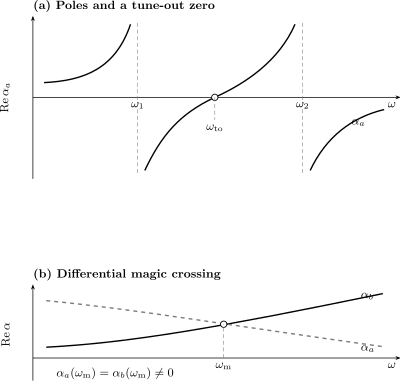
Schematic response, not data for a specific atom. Top: two resonances create dispersive poles and a zero of one state’s conservative response at $\omega_{\mathrm{to}}$. Bottom: a magic frequency $\omega_{\mathrm m}$ is a crossing of two state-dependent polarizabilities and need not occur at zero polarizability.

Plots require care:

• a wavelength axis reverses the ordering of a frequency axis;
• equal wavelength intervals are not equal frequency intervals;
• ideal poles should be excluded or replaced by a declared linewidth model;
• connecting points across a pole with a smooth line is unphysical;
• zeros and crossings should be found from the underlying function, not by reading a coarse plot.

Tune-Out Frequencies

A tune-out frequency for one specified state and geometry satisfies

$$\operatorname{Re} \alpha_a^{\mathrm{eff}} \left( \omega_{\mathrm{to}} \right) = 0.$$

At that frequency, the leading conservative electric-dipole potential of that state vanishes. The condition says nothing by itself about:

• $\operatorname{Im}\alpha$ and photon scattering;
• another internal state;
• higher multipoles;
• hyperpolarizability;
• spatial polarization gradients.

For two positive coefficients $C_1,C_2$ and $0<\omega_1<\omega_2$, consider

$$\alpha(\omega) = \frac{C_1}{\omega_1^2-\omega^2} + \frac{C_2}{\omega_2^2-\omega^2}.$$

the zero between the resonances is

$$\omega_{\mathrm{to}}^2 = \frac{ C_1\omega_2^2 + C_2\omega_1^2 }{ C_1+C_2 }.$$

This toy result makes the cancellation mechanism explicit. A measured tune-out frequency constrains a ratio of line strengths especially well, because an overall scale cancels from the root.

Precision tune-out measurements are also sensitive to effects omitted by a two-line model: higher excited states, core response, hyperfine structure, tensor response, polarization impurity, and continuum strength.

Magic Frequencies and Wavelengths

For a transition $|a\rangle\leftrightarrow|b\rangle$, define

$$\Delta\alpha_{ba}^{\mathrm{eff}}(\omega) = \alpha_b^{\mathrm{eff}}(\omega) - \alpha_a^{\mathrm{eff}}(\omega).$$

The leading differential light shift is

$$\delta\nu_{ba} = - \frac{ I }{ 2h\epsilon_0c } \operatorname{Re} \Delta\alpha_{ba}^{\mathrm{eff}}(\omega).$$

An electric-dipole magic frequency satisfies

$$\operatorname{Re} \Delta\alpha_{ba}^{\mathrm{eff}} \left( \omega_{\mathrm m} \right) = 0.$$

Unlike a tune-out condition, a magic crossing generally has

$$\alpha_a^{\mathrm{eff}}(\omega_{\mathrm m}) = \alpha_b^{\mathrm{eff}}(\omega_{\mathrm m}) \neq 0.$$

Both states can therefore remain trapped in the same nonzero optical potential while the leading differential shift cancels.

The corresponding vacuum wavelength is

$$\lambda_{\mathrm m} = \frac{ 2\pi c }{ \omega_{\mathrm m} }.$$

“Magic” is always conditional. It refers to specified:

• internal and motional states;
• polarization and propagation direction;
• quantization field;
• intensity regime;
• multipole order;
• experimental observable.

It does not automatically cancel vector or tensor shifts, magnetic-dipole or electric-quadrupole response, hyperpolarizability, motional state-dependence, or scattering.

Sensitivity to laser frequency

Near a simple magic root,

$$\operatorname{Re} \Delta\alpha(\omega) \simeq \left. \frac{ \partial\operatorname{Re}\Delta\alpha }{ \partial\omega } \right|_{\omega_{\mathrm m}} \left( \omega-\omega_{\mathrm m} \right).$$

The residual clock shift is therefore proportional to both intensity and laser-frequency error. A steep crossing can be easy to locate but demanding to operate; a shallow crossing is less frequency-sensitive but may carry a larger root uncertainty.

Computing a Trustworthy Polarizability

A reproducible calculation separates physics inputs from numerical bookkeeping.

1. Specify the observable

Record:

• isotope and internal state;
• $J$, $F$, and $m$ resolution;
• laser angular frequency or vacuum wavelength;
• polarization ellipse and propagation direction;
• quantization axis;
• peak, RMS, or intensity convention;
• whether the desired quantity is scalar, tensor-resolved, differential, real, imaginary, or complex.

2. Assemble energies

Use critically evaluated transition energies where available. The NIST Atomic Spectra Database supplies evaluated atomic energy levels, wavelengths, and transition probabilities, but its completeness and uncertainty vary by species and transition.

Measured energies are often much more accurate than calculated matrix elements. Replacing theoretical energies with evaluated values can improve denominators, provided this hybrid procedure is documented consistently.

3. Assemble matrix elements

Use reduced E1 matrix elements with one declared convention. Inputs may come from:

• high-precision many-body calculations;
• radiative lifetimes and branching fractions;
• oscillator-strength measurements;
• Stark-shift or tune-out measurements;
• internally consistent recommended compilations.

Because each scalar contribution is proportional to $|d|^2$,

$$\frac{ \delta\alpha_n }{ |\alpha_n| } \simeq 2 \frac{ \delta|d_{an}| }{ |d_{an}| }$$

when denominator uncertainty is negligible. Correlated matrix elements must not be varied independently.

4. Partition main, tail, core, and continuum

Compute dominant lines explicitly and estimate the remainder with a method appropriate to the atomic structure. Check that:

• no state appears in both main and tail pieces;
• Pauli-forbidden core transitions are removed consistently;
• continuum strength is represented;
• the chosen many-body method treats core polarization and valence correlation compatibly.

5. Apply angular reduction

Convert electronic reduced matrix elements to the required fine or hyperfine manifold using one Wigner–Eckart convention. Then contract with the actual polarization. Do not append vector and tensor “corrections” after a scalar calculation without checking normalization.

6. Evaluate away from singular points

Use frequency intervals that do not straddle unresolved poles. Near a resonance, include a physical linewidth or replace the perturbative model. For a tabulation in wavelength, perform the calculation in $\omega$ and transform the independent variable only for output.

7. Run consistency checks

Useful checks include:

1. $\alpha(0)$ agrees with the static calculation;
2. $\alpha(-\omega)=\alpha(\omega)^*$;
3. the high-frequency tail has the expected sign and scaling;
4. length- and velocity-gauge matrix elements converge toward agreement;
5. basis enlargement stabilizes tail and continuum contributions;
6. the scalar response is independent of $m$;
7. vector and tensor reversals follow their symmetry signatures;
8. removing one dominant line changes the result by its tabulated contribution.

Gauge disagreement in a truncated atomic-structure calculation is a diagnostic of incompleteness, not a physical uncertainty to be hidden by averaging the gauges.

8. Propagate uncertainty and covariance

For input parameters $x_i$ with covariance matrix $C_{ij}$,

$$\sigma_\alpha^2 = \sum_{ij} \frac{\partial\alpha}{\partial x_i} C_{ij} \frac{\partial\alpha}{\partial x_j}.$$

Near cancellation, quote absolute uncertainty as well as relative uncertainty. The latter can diverge at a perfectly well-defined zero.

For a simple tune-out root,

$$\delta\omega_{\mathrm{to}} \simeq - \frac{ \delta\alpha(\omega_{\mathrm{to}}) }{ \left. \partial_\omega\alpha \right|_{\omega_{\mathrm{to}}} }.$$

For a magic root, replace $\alpha$ by $\Delta\alpha$. Monte Carlo sampling is preferable when inputs are non-Gaussian, roots exchange order, or the linearization is poor.

Optical Trapping

For a slowly varying monochromatic field, the state-dependent electric-dipole potential is

$$U_a(\mathbf r) = - \frac{ I(\mathbf r) }{ 2\epsilon_0c } \operatorname{Re} \alpha_a^{\mathrm{eff}} \left( \omega,\mathbf r \right).$$

The spatial argument on $\alpha_a^{\mathrm{eff}}$ allows for polarization gradients and a position-dependent quantization axis. The conservative dipole force is

$$\mathbf F_{\mathrm{dip}} = - \boldsymbol\nabla U_a.$$

If the effective polarizability is spatially uniform,

$$\mathbf F_{\mathrm{dip}} = \frac{ \operatorname{Re}\alpha_a^{\mathrm{eff}} }{ 2\epsilon_0c } \boldsymbol\nabla I.$$

Thus:

• positive polarizability attracts the state toward intensity maxima;
• negative polarizability repels it toward intensity minima;
• a tune-out state has no leading scalar gradient force;
• polarization gradients can still create vector or tensor forces.

The dissipative radiation-pressure and momentum-diffusion forces are not generated by this conservative potential. They require the imaginary response and the photon momentum distribution.

Gaussian-beam trap frequencies

At the waist of a circular Gaussian beam,

$$I(r,0) = I_0 \exp \left( - \frac{2r^2}{w_0^2} \right).$$

For a red-seeking state with $\operatorname{Re}\alpha>0$, define

$$U_0 = - \frac{ \operatorname{Re}\alpha I_0 }{ 2\epsilon_0c } < 0.$$

Near the center,

$$U(r,0) \simeq U_0 + \frac{ 2|U_0| }{ w_0^2 } r^2.$$

For particle mass $M$, the radial angular frequency is

$$\omega_r = \sqrt{ \frac{ 4|U_0| }{ Mw_0^2 } }.$$

With Rayleigh range

$$z_R = \frac{ \pi w_0^2 }{ \lambda },$$

the on-axis intensity obeys

$$I(0,z) \simeq I_0 \left( 1-\frac{z^2}{z_R^2} \right),$$

and the axial angular frequency is

$$\omega_z = \sqrt{ \frac{ 2|U_0| }{ Mz_R^2 } }.$$

These formulas neglect gravity, astigmatism, standing-wave structure, aberrations, and state-dependent polarization. They are curvature checks, not complete trap models.

Numerical scale

Take

$$\begin{gathered} \operatorname{Re}\alpha = 300\ \mathrm{a.u.}, \\ I_0 = 1.00\times10^8\ \mathrm{W\,m^{-2}}, \\ w_0 = 30.0\ \mu\mathrm m, \\ \lambda = 1064\ \mathrm{nm}, \end{gathered}$$

and $M=88\,\mathrm u$. The central potential is

$$\frac{U_0}{h} \simeq - 1.41\times10^5\ \mathrm{Hz},$$

or

$$\frac{U_0}{k_{\mathrm B}} \simeq - 6.75\ \mu\mathrm K.$$

The ideal harmonic frequencies are

$$\frac{\omega_r}{2\pi} \simeq 268\ \mathrm{Hz}, \qquad \frac{\omega_z}{2\pi} \simeq 2.14\ \mathrm{Hz}.$$

The large aspect ratio is a geometric consequence of $z_R\gg w_0$.

State-dependent confinement

Two internal states with different polarizabilities experience different trap depths and vibrational frequencies. Even if their bare internal transition is narrow, this can produce:

• motional-state-dependent line shifts;
• inhomogeneous broadening across a thermal ensemble;
• entanglement between internal and motional degrees of freedom;
• dephasing when atoms sample different intensities;
• imperfect overlap in state-changing collisions or gates.

A magic condition suppresses the leading differential E1 potential. It does not guarantee identical loss rates or identical higher-order confinement.

Tune-out is not loss-out

At a tune-out frequency,

$$\operatorname{Re}\alpha(\omega_{\mathrm{to}}) = 0,$$

but generally

$$\operatorname{Im}\alpha(\omega_{\mathrm{to}}) \neq 0.$$

The leading conservative potential may vanish while recoil heating, spontaneous Raman transitions, or photoionization remains. A useful trap wavelength therefore requires evaluating the complex response, not only its real zero.

Optical Clocks and Differential Response

For clock states $|g\rangle$ and $|e\rangle$,

$$\delta\nu_{\mathrm{clock}} = - \frac{ I }{ 2h\epsilon_0c } \operatorname{Re} \left[ \alpha_e^{\mathrm{eff}}(\omega) - \alpha_g^{\mathrm{eff}}(\omega) \right].$$

At an electric-dipole magic frequency, the bracket vanishes to leading order. This permits confinement while suppressing the dominant intensity-dependent clock shift.

Intensity and frequency noise

Away from a magic point,

$$\frac{ \partial\delta\nu_{\mathrm{clock}} }{ \partial I } = - \frac{ \operatorname{Re}\Delta\alpha }{ 2h\epsilon_0c }.$$

At a simple magic point, the first-order intensity coefficient vanishes, but laser-frequency fluctuations restore a differential coefficient:

$$\delta\nu_{\mathrm{clock}} \simeq - \frac{ I }{ 2h\epsilon_0c } \left. \frac{ \partial\operatorname{Re}\Delta\alpha }{ \partial\omega } \right|_{\omega_{\mathrm m}} \delta\omega_L.$$

An operational uncertainty budget therefore needs both intensity and frequency calibration, including their possible correlation.

Beyond the leading magic condition

A useful local expansion is

$$\delta\nu = \kappa_1(\omega)I + \kappa_2(\omega)I^2 + \cdots.$$

The E1 magic condition sets the relevant part of $\kappa_1$ to zero. The coefficient $\kappa_2$ can contain hyperpolarizability and multiphoton effects. Additional residuals include:

• magnetic-dipole and electric-quadrupole lattice couplings;
• vector shifts from ellipticity;
• tensor shifts from alignment;
• motional averaging and tunneling;
• spatial polarization structure;
• probe-light shifts during interrogation;
• collisions and density-dependent shifts.

The magic wavelength proposed for optical lattice clocks is therefore a controlled cancellation, not a claim that the atom is unperturbed by light.

Differential scattering

Even when

$$\operatorname{Re}\alpha_e = \operatorname{Re}\alpha_g,$$

one may have

$$\operatorname{Im}\alpha_e \neq \operatorname{Im}\alpha_g.$$

Different Raman-scattering channels can reveal which-path information and dephase a clock or qubit superposition. State-insensitive conservative trapping does not imply state-insensitive dissipation.

Broadband Fields and Thermal Radiation

Dynamic polarizability also organizes response to an incoherent spectrum. Let a one-sided electric-field spectral density be normalized by

$$\left\langle E^2\right\rangle = \int_0^\infty d\omega\, S_E(\omega).$$

For an isotropic scalar state in the weak-response regime,

$$\delta E_a = - \frac12 \int_0^\infty d\omega\, S_E(\omega) \operatorname{Re}\alpha_a(\omega).$$

Approximating $\alpha_a(\omega)$ by $\alpha_a(0)$ gives the leading static blackbody-radiation shift. Precision work requires the dynamic correction from the thermal spectrum and a measured electromagnetic environment.

Blackbody Radiation develops the Planck spectrum; Precision Spectroscopy owns the experimental temperature, emissivity, and view-factor budget.

Measuring Dynamic Polarizability

Different experiments constrain different combinations of the response:

• Light shift versus intensity: differential $\operatorname{Re}\alpha$, limited by local intensity calibration.
• Trap oscillation frequency: curvature of the absolute potential, limited by beam geometry and anharmonicity.
• Atom-interferometer phase: path-integrated differential $U/\hbar$, limited by wave-packet overlap.
• Kapitza–Dirac diffraction: short-pulse optical potential, limited by pulse area and lattice contrast.
• Tune-out zero: ratio of competing contributions, limited by polarization and residual forces.
• Photon scattering or loss: $\operatorname{Im}\alpha$ and branching, limited by collection and channel modeling.
• Absorption spectrum: spectral strength, limited by saturation and the line-shape model.

Intensity calibration

Inferring an absolute polarizability from a light shift requires the intensity at the atom, not merely laser power upstream. The calibration depends on:

• waist and aberrations;
• standing-wave contrast;
• window transmission;
• polarization at the atom;
• atomic position and thermal distribution;
• temporal pulse envelope.

Ratios, zeros, and crossings can suppress some common calibration errors, which is one reason tune-out and magic measurements are powerful tests of atomic structure.

Sign determination

A trap frequency determines a curvature magnitude unless the direction of the force is also known. The sign of $\operatorname{Re}\alpha$ can be identified by:

• attraction toward or repulsion from an intensity maximum;
• interferometric phase relative to a calibrated reference;
• the direction of a measured light shift;
• continuity from a known side of a resonance.

Polarization control

At high precision, characterize polarization after the final vacuum window or infer it in situ. Stress birefringence can make a nominally linear beam elliptical. Reversing helicity and magnetic sublevel helps diagnose vector response; rotating the bias field diagnoses tensor response.

Frequency calibration

Quote vacuum frequency or vacuum wavelength and the calibration chain. Air wavelength depends on refractive index. Near a steep zero or crossing, the difference can be much larger than the target uncertainty.

Regime Map

Regime	Appropriate description
far from every line, weak drive	real sum-over-states polarizability
weak drive near an isolated broadened line	complex linear response
appreciable saturation	optical Bloch equations
coherent strong coupling	dressed-state or Floquet eigenproblem
several nearby levels	multilevel response or direct diagonalization
above ionization threshold	continuum response and photoionization
intense field with nonlinear shift	hyperpolarizability or nonperturbative model
structured photonic environment	environment-dependent Green tensor

The word “off-resonant” is not sufficient. A reliable model compares detunings, linewidths, Rabi frequencies, neighboring level spacings, interaction time, and the required accuracy.

Common Mistakes

Keeping only the nearest line everywhere

A nearest-line model may estimate a far-detuned shift locally, but it cannot reliably predict tune-out zeros, magic crossings, static response, or high-frequency asymptotics.

Dropping the counter-rotating denominator globally

The rotating-wave term is controlled near one positive-frequency resonance. The complete dynamic polarizability contains both signs of the drive frequency.

Omitting continuum or core response

Small background terms can move a cancellation point substantially even when they barely change the polarizability away from the root.

Treating an ideal pole as a finite prediction

An infinite perturbative value signals breakdown. Insert a physically justified width or switch to a resonant dynamical model.

Calling every zero magic

A tune-out zero cancels one state’s response. A magic crossing cancels the difference between two states. They are distinct conditions.

Assuming magic means no scattering

The real differential response can vanish while either state retains a nonzero imaginary response and state-changing Raman channels.

Ignoring polarization and magnetic sublevel

Scalar, vector, and tensor terms can move both tune-out and magic wavelengths. The required metadata are part of the result.

Mixing angular frequency and ordinary frequency

The denominators use $\omega$ in radians per second. Replacing it with $\nu$ without converting $\omega=2\pi\nu$ moves every pole.

Mixing peak and RMS fields

The peak-field light shift contains $1/4$; the RMS-field expression contains $1/2$.

Plotting through a resonance

A line joining samples on opposite sides of a pole invents finite values that the model never predicted.

Quoting only relative uncertainty at a zero

Relative uncertainty is ill-conditioned when the central value vanishes. Quote absolute response uncertainty and root uncertainty.

Ignoring covariance

Matrix elements inferred from shared lifetimes, branching ratios, or theory parameters are correlated. Independent error bars can overestimate or underestimate the uncertainty of a cancellation.

Key Results

1. Dynamic polarizability is a causal, generally complex response tensor.
2. Its spectral sum contains rotating and counter-rotating denominators.
3. Discrete, continuum, core, and tail contributions belong to one complete response.
4. $\operatorname{Re}\alpha$ determines the leading conservative light shift; $\operatorname{Im}\alpha$ determines weak dissipative response.
5. Scalar, vector, and tensor components have distinct reversal signatures.
6. A tune-out frequency solves $\operatorname{Re}\alpha_a=0$ for one state.
7. A magic frequency solves $\operatorname{Re}(\alpha_b-\alpha_a)=0$ for a transition.
8. A magic crossing can retain a nonzero common trapping potential.
9. Near a cancellation, small omitted terms and correlated uncertainties can dominate the root location.
10. Poles require resonant dynamics; they are not finite trap predictions.

Further Connections

• AC Stark Shift derives the two-level shift and its virtual-admixture interpretation.
• Optical Dipole Traps uses state-resolved polarizabilities to calculate confinement, differential shifts, scattering, and technical error budgets.
• Stark Effect in Atoms compares static and oscillating electric response in real atomic manifolds.
• Optical Bloch Equations replaces linear response near a saturated dissipative resonance.
• Radiation Pressure develops the mechanical force associated with absorptive response and contrasts it with the dispersive dipole force.
• Oscillator Strengths supplies the data dictionary among matrix elements, lifetimes, and line strengths.
• Raman Spectroscopy uses a geometry-dependent polarizability tensor for two-photon response.
• Transition Rates in Light–Matter Interaction develops the rate interpretation of absorptive spectral strength.
• Precision Spectroscopy turns differential polarizabilities into calibrated systematic corrections.
• Optical Clocks applies differential static and dynamic polarizabilities to magic trapping, blackbody shifts, and clock uncertainty budgets.

References

1. J. Mitroy, M. S. Safronova, and C. W. Clark, “Theory and applications of atomic and ionic polarizabilities,” Journal of Physics B 43, 202001 (2010); arXiv:1004.3567.
2. N. L. Manakov, V. D. Ovsiannikov, and L. P. Rapoport, “Atoms in a laser field,” Physics Reports 141, 320–433 (1986).
3. F. Le Kien, P. Schneeweiss, and A. Rauschenbeutel, “Dynamical polarizability of atoms in arbitrary light fields: general theory and application to cesium,” European Physical Journal D 67, 92 (2013); arXiv:1211.2673.
4. M. S. Safronova, B. Arora, and C. W. Clark, “Frequency-dependent polarizabilities of alkali-metal atoms from ultraviolet through infrared spectral regions,” Physical Review A 73, 022505 (2006).
5. B. Arora, M. S. Safronova, and C. W. Clark, “Magic wavelengths for the $np$–$ns$ transitions in alkali-metal atoms,” Physical Review A 76, 052509 (2007).
6. R. Grimm, M. Weidemüller, and Y. B. Ovchinnikov, “Optical Dipole Traps for Neutral Atoms,” Advances in Atomic, Molecular, and Optical Physics 42, 95–170 (2000); arXiv:physics/9902072.
7. H. Katori, M. Takamoto, V. G. Pal’chikov, and V. D. Ovsiannikov, “Ultrastable Optical Clock with Neutral Atoms in an Engineered Light Shift Trap,” Physical Review Letters 91, 173005 (2003).
8. B. M. Henson, R. I. Khakimov, R. G. Dall, K. G. H. Baldwin, Li-Yan Tang, and A. G. Truscott, “Precision Measurement for Metastable Helium Atoms of the 413 nm Tune-Out Wavelength at Which the Atomic Polarizability Vanishes,” Physical Review Letters 115, 043004 (2015).
9. R. H. Leonard, A. J. Fallon, C. A. Sackett, and M. S. Safronova, “High-precision measurements of the $^{87}\mathrm{Rb}$ D-line tune-out wavelength,” Physical Review A 92, 052501 (2015).
10. F. Schmidt, D. Mayer, M. Hohmann, T. Lausch, F. Kindermann, and A. Widera, “Precision measurement of the $^{87}\mathrm{Rb}$ tune-out wavelength in the hyperfine ground state $F=1$ at 790 nm,” Physical Review A 93, 022507 (2016).
11. M. S. Safronova, U. I. Safronova, and C. W. Clark, “Magic wavelengths, matrix elements, polarizabilities, and lifetimes of Cs,” Physical Review A 94, 012505 (2016).
12. A. Kramida, Yu. Ralchenko, J. Reader, and NIST ASD Team, NIST Atomic Spectra Database, version 5.12, National Institute of Standards and Technology (2024).
13. E. Tiesinga, P. J. Mohr, D. B. Newell, and B. N. Taylor, “CODATA recommended values of the fundamental physical constants: 2022,” Journal of Physical and Chemical Reference Data 54, 033105 (2025).
14. C. Cohen-Tannoudji, J. Dupont-Roc, and G. Grynberg, Atom–Photon Interactions: Basic Processes and Applications (Wiley, 1992).

Exercises

1. Recover the far-detuned two-level shift

For one ground-to-excited transition, start from

$$\alpha_g(\omega) = \frac{|d_{eg}|^2}{\hbar} \left[ \frac1{\omega_0-\omega} + \frac1{\omega_0+\omega} \right].$$

Combine the denominators. Then take the near-resonant but far-detuned limit $|\Delta|\ll\omega_0$ and $|\Delta|\gg|\Omega|,\Gamma$, where $\Delta=\omega_0-\omega$ and $\Omega=E_0|d_{eg}|/\hbar$. Show that the light shift agrees with the two-level result.

Solution

Combining denominators gives

$$\begin{aligned} \alpha_g(\omega) &= \frac{|d_{eg}|^2}{\hbar} \frac{ 2\omega_0 }{ \omega_0^2-\omega^2 } \\ &= \frac{ 2\omega_0|d_{eg}|^2 }{ \hbar \left( \omega_0^2-\omega^2 \right) }. \end{aligned}$$

Near the positive-frequency resonance,

$$\omega_0+\omega \simeq 2\omega_0,$$

so

$$\alpha_g(\omega) \simeq \frac{ |d_{eg}|^2 }{ \hbar\Delta }.$$

The peak-field light shift is

$$\begin{aligned} U_g &= - \frac14 \alpha_gE_0^2 \\ &\simeq - \frac{ E_0^2|d_{eg}|^2 }{ 4\hbar\Delta } \\ &= - \frac{ \hbar|\Omega|^2 }{ 4\Delta }. \end{aligned}$$

This is the far-detuned ground-state branch in the stated atom-minus-laser detuning convention.

2. Locate a two-line tune-out frequency

Let

$$\alpha(\omega) = \frac1{1-\omega^2} + \frac3{4-\omega^2},$$

where all frequencies are in the same arbitrary units. Find the tune-out frequency between the poles and verify the signs of the two contributions there.

Solution

For

$$C_1=1, \quad C_2=3, \quad \omega_1=1, \quad \omega_2=2,$$

the general root gives

$$\omega_{\mathrm{to}}^2 = \frac{ (1)(4)+(3)(1) }{ 1+3 } = \frac74.$$

Therefore

$$\omega_{\mathrm{to}} = \frac{\sqrt7}{2} \simeq 1.323,$$

which lies between $1$ and $2$.

At this frequency,

$$\frac1{1-\omega_{\mathrm{to}}^2} = - \frac43,$$

while

$$\frac3{4-\omega_{\mathrm{to}}^2} = \frac43.$$

The zero comes from cancellation, not from either transition becoming irrelevant.

3. Use the oscillator-strength sum rule

Starting from

$$\alpha(\omega) = \frac{e^2}{m_e} \sum_n \frac{ f_{an} }{ \omega_{na}^2-\omega^2 },$$

derive the leading high-frequency behavior for an $N$-electron atom. Explain what a coefficient corresponding to $N_{\mathrm{eff}}<N$ indicates in a truncated calculation.

Solution

For $|\omega|\gg|\omega_{na}|$,

$$\frac1{ \omega_{na}^2-\omega^2 } = - \frac1{\omega^2} + O(\omega^{-4}).$$

Hence

$$\alpha(\omega) = - \frac{e^2}{m_e\omega^2} \sum_n f_{an} + O(\omega^{-4}).$$

Using the Thomas–Reiche–Kuhn sum rule,

$$\sum_n f_{an} = N,$$

gives

$$\alpha(\omega) \sim - \frac{ Ne^2 }{ m_e\omega^2 }.$$

If the numerical coefficient corresponds to $N_{\mathrm{eff}}<N$, oscillator strength is missing from the represented spectrum. Common causes are omitted continuum states, an incomplete basis, or a core model whose contribution has not been restored. In an effective Hamiltonian, the comparison must use the electron count represented by that model and its consistent effective operators.

4. Recover the shift–scattering ratio

Near one weak broadened line, use

$$\alpha(\omega) \simeq \frac{ D }{ \Delta-i\Gamma/2 }, \qquad D = \frac{|d_{eg}|^2}{\hbar}.$$

Find its real and imaginary parts and show that far from resonance

$$\frac{ \hbar\Gamma_{\mathrm{sc}} }{ |U| } \simeq \frac{\Gamma}{|\Delta|}.$$

Solution

Multiplying by the complex conjugate denominator gives

$$\operatorname{Re}\alpha = \frac{ D\Delta }{ \Delta^2+\Gamma^2/4 },$$

and

$$\operatorname{Im}\alpha = \frac{ D\Gamma/2 }{ \Delta^2+\Gamma^2/4 }.$$

The general weak-response ratio is

$$\frac{ \hbar\Gamma_{\mathrm{sc}} }{ |U| } = 2 \frac{ \operatorname{Im}\alpha }{ |\operatorname{Re}\alpha| }.$$

Therefore

$$\frac{ \hbar\Gamma_{\mathrm{sc}} }{ |U| } = \frac{\Gamma}{|\Delta|}.$$

The result actually follows for this single-pole model at any nonzero $\Delta$; calling it far-detuned additionally ensures weak excitation and the validity of the conservative-potential picture.

At $\Delta=0$, the real part vanishes while absorption is maximal. That is not a useful tune-out point because the linear resonant model is strongly dissipative.

5. Estimate Gaussian trap frequencies

Use

$$\begin{gathered} \operatorname{Re}\alpha = 300\ \mathrm{a.u.}, \\ I_0 = 1.00\times10^8\ \mathrm{W\,m^{-2}}, \end{gathered}$$

for a particle of mass $88\,\mathrm u$ in a Gaussian beam with

$$w_0 = 30.0\ \mu\mathrm m, \qquad \lambda = 1064\ \mathrm{nm}.$$

Compute $U_0/h$, $U_0/k_{\mathrm B}$, and the radial and axial trap frequencies. Neglect gravity and aberrations.

Solution

Let $\alpha_{\mathrm{au}}$ denote one atomic unit of polarizability. Then

$$\begin{aligned} \alpha &= 300\alpha_{\mathrm{au}} \\ &= 4.9463\times10^{-39} \frac{ \mathrm{C^2\,m^2} }{ \mathrm J }. \end{aligned}$$

The central depth is

$$U_0 = - \frac{ \alpha I_0 }{ 2\epsilon_0c } = - 9.32\times10^{-29}\ \mathrm J.$$

Therefore

$$\frac{U_0}{h} \simeq - 1.41\times10^5\ \mathrm{Hz},$$

and

$$\frac{U_0}{k_{\mathrm B}} \simeq - 6.75\ \mu\mathrm K.$$

The mass and Rayleigh range are

$$M = 88\,\mathrm u \simeq 1.4613\times10^{-25}\ \mathrm{kg},$$

and

$$z_R = \frac{\pi w_0^2}{\lambda} \simeq 2.657\times10^{-3}\ \mathrm m.$$

The radial result is

$$\frac{\omega_r}{2\pi} = \frac1{2\pi} \sqrt{ \frac{ 4|U_0| }{ Mw_0^2 } } \simeq 268\ \mathrm{Hz}.$$

The axial result is

$$\frac{\omega_z}{2\pi} = \frac1{2\pi} \sqrt{ \frac{ 2|U_0| }{ Mz_R^2 } } \simeq 2.14\ \mathrm{Hz}.$$

6. Find a magic crossing and its residual

Near a candidate frequency, suppose two scalar polarizabilities in atomic units are modeled by

$$\alpha_a = 100+2x, \qquad \alpha_b = 130-x,$$

where $x$ is a dimensionless calibrated frequency offset. Find the magic point and the common polarizability. If the experiment operates at $x=x_{\mathrm m}+0.20$, find $\Delta\alpha=\alpha_b-\alpha_a$.

Solution

The crossing satisfies

$$100+2x_{\mathrm m} = 130-x_{\mathrm m}.$$

Hence

$$x_{\mathrm m} = 10.$$

Both states then have

$$\alpha_a = \alpha_b = 120\ \mathrm{a.u.}$$

The trap is magic but not tuned out.

The differential response is

$$\Delta\alpha = 30-3x.$$

At $x=10.20$,

$$\Delta\alpha = - 0.60\ \mathrm{a.u.}$$

The sign predicts an upward transition-frequency shift in the peak-field convention because $\delta\nu=-I\Delta\alpha/(2h\epsilon_0c)$.

7. Separate vector and tensor shifts

Suppose the tensor geometry factor is

$$\begin{aligned} Q(m,\theta) &= \left( 3\cos^2\theta-1 \right) \\ &\quad\times \left[ 3m^2-F(F+1) \right]. \end{aligned}$$

A measured frequency has the form

$$\nu(m,\mathcal A,\theta) = \nu_{\mathrm s} + \mathcal A m\,\nu_{\mathrm v} + Q(m,\theta) \nu_{\mathrm t},$$

where normalization constants have been absorbed into $\nu_{\mathrm v}$ and $\nu_{\mathrm t}$. Which reversals isolate the vector term? How can the tensor term be distinguished from the scalar term?

Solution

At fixed helicity and angle,

$$\frac{ \nu(+m,\mathcal A,\theta) - \nu(-m,\mathcal A,\theta) }{ 2 } = \mathcal A m\,\nu_{\mathrm v}.$$

This isolates the vector response because the scalar and tensor terms are even in $m$. Helicity reversal gives an independent vector estimator:

$$\frac{ \nu(m,+1,\theta) - \nu(m,-1,\theta) }{ 2 } = m\,\nu_{\mathrm v}.$$

Averaging either reversal pair removes the vector term. The remaining scalar and tensor terms can be separated by changing $|m|$ or rotating the linear polarization relative to the quantization axis. In particular, the tensor geometry factor vanishes at the magic angle satisfying

$$3\cos^2\theta-1 = 0,$$

or

$$\cos^2\theta = \frac13.$$

Comparing this orientation with another angle separates the scalar offset from the tensor dependence. Real experiments must also account for ellipticity and imperfect magnetic-state preparation.

8. Propagate uncertainty to a tune-out root

For the two-line model of Exercise 2, let

$$C_1 = 1.00\pm0.01, \qquad C_2 = 3.00\pm0.06,$$

with exact $\omega_1=1$, $\omega_2=2$ and initially uncorrelated coefficient uncertainties. Estimate the uncertainty in $\omega_{\mathrm{to}}$. What happens to the root if both $C_1$ and $C_2$ share the same fractional scale error?

Solution

Let

$$x = \omega_{\mathrm{to}}^2 = \frac{ C_1\omega_2^2 + C_2\omega_1^2 }{ C_1+C_2 }.$$

At the central values,

$$x = \frac74.$$

The derivatives are

$$\frac{\partial x}{\partial C_1} = \frac{ C_2 \left( \omega_2^2-\omega_1^2 \right) }{ \left( C_1+C_2 \right)^2 } = \frac9{16},$$

and

$$\frac{\partial x}{\partial C_2} = \frac{ C_1 \left( \omega_1^2-\omega_2^2 \right) }{ \left( C_1+C_2 \right)^2 } = - \frac3{16}.$$

For uncorrelated inputs,

$$\begin{aligned} \sigma_x^2 &= \left( \frac9{16} \right)^2 (0.01)^2 \\ &\quad + \left( \frac3{16} \right)^2 (0.06)^2. \end{aligned}$$

Therefore

$$\sigma_x \simeq 0.0126.$$

Since $\omega_{\mathrm{to}}=\sqrt{x}$,

$$\sigma_{\omega} = \frac{ \sigma_x }{ 2\sqrt{x} } \simeq 0.0048.$$

Thus

$$\omega_{\mathrm{to}} = 1.3229\pm0.0048$$

in the model’s frequency units.

If both coefficients acquire the same fractional scale factor,

$$C_i \longrightarrow sC_i,$$

that factor cancels exactly from $x$. A common normalization uncertainty does not move this ideal tune-out root. Treating the two coefficients as independent would miss that covariance and overstate the root uncertainty.