Optical Dipole Traps

An optical dipole trap confines a polarizable particle through the position-dependent AC Stark shift produced by an inhomogeneous light field. For an atom in internal state $|a\rangle$, the center-of-mass Hamiltonian is approximately

$$H_{\mathrm{cm},a} = \frac{\mathbf p^2}{2m} + U_a(\mathbf r),$$

where $U_a(\mathbf r)$ is the light-shift energy of the adiabatically followed internal state. The mechanical force is

$$\mathbf F_a(\mathbf r) = -\boldsymbol{\nabla}U_a(\mathbf r).$$

Unlike a magneto-optical trap, an ideal dipole trap does not need resonant photon scattering to provide either confinement or damping. It is therefore called conservative. Real dipole traps are only approximately conservative: off-resonant scattering, technical noise, background collisions, internal-state changes, and finite trap depth all produce heating or loss.

The useful question is not merely whether a laser shifts an atomic level. One must separately establish:

1. the sign and spatial shape of the potential;
2. the curvature and finite escape barriers;
3. the photon-scattering and technical-heating rates;
4. the internal-state dependence;
5. the loading and loss budget.

A deep trap can have poor coherence. A low-scattering light field can fail to support atoms against gravity. A large harmonic frequency can coexist with a small escape depth. These are distinct measurements.

Canonical Scope

This page owns the center-of-mass mechanics of optical dipole traps:

1. conversion of a dynamic polarizability into an optical potential;
2. the far-detuned two-level limit and its regime of validity;
3. bright, red-detuned and dark, blue-detuned trapping;
4. Gaussian-beam trap depths, curvatures, and normal-mode frequencies;
5. photon-scattering, recoil-heating, and detuning tradeoffs;
6. gravity, anharmonicity, loading, technical noise, and loss;
7. state-dependent trapping, magic conditions, and experimental calibration.

AC Stark Shift owns the dressed-state derivation of the light shift. Dynamic Polarizability owns the full sum over atomic levels, scalar-vector-tensor decomposition, tune-out frequencies, and magic crossings. This page uses those results as inputs to a mechanical trap model rather than repeating their derivations.

Magneto-Optical Traps owns dissipative capture and precooling. Radiation Pressure owns the resonant scattering force. Optical Tweezers specializes the same potential to single-particle loading, imaging, and rearrangeable arrays. Evaporative Cooling owns energy-selective loss and rethermalization after trap loading. Later pages treat lattices and ultracold gases.

Conventions and Validity

Write a monochromatic electric field as

$$\mathbf E(\mathbf r,t) = \operatorname{Re} \left[ E_0(\mathbf r) \boldsymbol{\epsilon}(\mathbf r) e^{-i\omega_Lt} \right],$$

where $E_0$ is the peak field amplitude and $\boldsymbol{\epsilon}^{\,*}\mathbin{\cdot}\boldsymbol{\epsilon}=1$. The cycle-averaged intensity in vacuum is

$$I(\mathbf r) = \frac{1}{2} \epsilon_0c |E_0(\mathbf r)|^2.$$

For a passive atom, define the effective polarizability in state $|a\rangle$ by

$$\alpha_a^{\mathrm{eff}} = \boldsymbol{\epsilon}^{\,*} \mathbin{\cdot} \boldsymbol{\alpha}_a(\omega_L) \mathbin{\cdot} \boldsymbol{\epsilon}.$$

This quantity may depend on position if the polarization, quantization axis, or internal eigenstate varies.

For a two-level comparison, use atom-minus-laser detuning

$$\Delta = \omega_0-\omega_L.$$

Thus:

• red detuning has $\Delta>0$;
• blue detuning has $\Delta<0$.

This sign convention is opposite to the commonly used $\Delta_L=\omega_L-\omega_0$. A formula imported from another source must be translated before its sign is interpreted.

Hierarchy of approximations

The simplest dipole-potential model assumes:

$$|\Delta| \gg \Gamma, \qquad |\Delta| \gg |\Omega|, \qquad s_{\mathrm{eff}} \ll 1,$$

where $\Gamma$ is the natural linewidth, $\Omega$ is the local resonant Rabi frequency, and $s_{\mathrm{eff}}$ is the detuning-reduced saturation parameter. These conditions suppress real excited-state population and power broadening.

Additional checks are separate:

• Atomic structure: a two-level reduction is unreliable when several fine-structure, hyperfine, molecular, or continuum channels contribute.
• Adiabatic internal following: motion through polarization or intensity gradients must not drive transitions between local dressed states.
• Slow envelope: the optical cycle is much faster than the center-of-mass motion, allowing a cycle-averaged potential.
• Coherent beams: fields at the same frequency and polarization may interfere. Their electric fields must be added before converting to intensity.
• Incoherent or rapidly dephased beams: their time-averaged potentials can usually be added.

The term far detuned is therefore relative to all nearby resonances that matter, not only to one selected line.

From Polarizability to a Potential

With the field convention above, the conservative light shift is

$$U_a(\mathbf r) = - \frac{1}{4} \operatorname{Re} \alpha_a^{\mathrm{eff}}(\omega_L) |E_0(\mathbf r)|^2.$$

Equivalently,

$$U_a(\mathbf r) = - \frac{ \operatorname{Re} \alpha_a^{\mathrm{eff}}(\omega_L) }{ 2\epsilon_0c } I(\mathbf r).$$

For spatially uniform polarizability,

$$\mathbf F_a = \frac{ \operatorname{Re}\alpha_a^{\mathrm{eff}} }{ 2\epsilon_0c } \boldsymbol{\nabla}I.$$

A positive real polarizability pulls the atom toward higher intensity. A negative real polarizability pushes it toward lower intensity. If the local polarization changes, the force must instead be calculated from the gradient of the complete eigenenergy $U_a(\mathbf r)$; differentiating intensity alone can miss vector and tensor light-shift forces.

Far-detuned two-level form

For a ground state in the rotating-wave and weak-excitation limits,

$$U_g(\mathbf r) \simeq - \frac{ \hbar|\Omega(\mathbf r)|^2 }{ 4\Delta }.$$

The excited-state admixture is of order

$$P_e \simeq \frac{ |\Omega|^2 }{ 4\Delta^2 }.$$

Consequently, the conservative force survives even when the instantaneous excited-state population is very small. The atom is not being pulled because it repeatedly absorbs photons from the high-intensity side. The force is the gradient of a dressed-state energy.

For an alkali atom, a single detuning is often inadequate. The D1 and D2 lines can contribute with different weights, and the vector and tensor parts depend on hyperfine state, polarization, and magnetic field. Near a cancellation between contributions, the potential may be small while the scattering rate remains appreciable. The full dynamic-polarizability calculation is then mandatory.

Red and Blue Detuning

In the ideal two-level ground-state model,

$$\begin{array}{c|c|c} \text{detuning} & U_g & \text{preferred region} \\ \hline \Delta>0\ \text{(red)} & U_g<0 & \text{high intensity} \\ \Delta<0\ \text{(blue)} & U_g>0 & \text{low intensity} \end{array}$$

Red-detuned bright traps

A focused red-detuned beam produces a negative potential whose minimum is at the intensity maximum. If the potential tends to zero far from the beam and the minimum is $-U_0$, then $U_0>0$ is the nominal trap depth in the absence of gravity or other fields.

Bright traps are simple and provide strong curvature for a given optical geometry. Their main disadvantage is that trapped particles reside where the intensity, AC Stark shift, and scattering rate are largest.

Blue-detuned dark traps

Blue-detuned light produces positive energy where the intensity is high. Particles seek an intensity minimum. A single focused blue-detuned Gaussian beam is a barrier, not a three-dimensional trap. Confinement requires a dark region surrounded by bright walls, for example a hollow beam, a bottle beam, crossed light sheets, or an interference pattern.

A dark trap can reduce the average scattering and differential light shift because a cold particle spends most of its time near low intensity. Nevertheless, the barrier height, tunneling or escape channels, residual intensity at the minimum, and nonadiabatic polarization structure must all be checked.

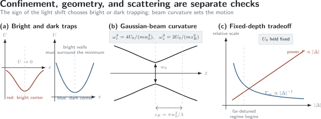
Red detuning gives a bright-centered well, whereas blue detuning requires an engineered dark minimum enclosed by optical barriers. A Gaussian beam has much stronger radial than axial curvature when $z_R\gg w_0$. In the ideal two-level far-detuned limit, maintaining fixed depth while increasing $|\Delta|$ requires power proportional to $|\Delta|$, but reduces the scattering rate as $|\Delta|^{-1}$.

A Single Gaussian-Beam Trap

Let $\rho^2=x^2+y^2$ measure distance from the propagation axis $z$. A TEM$_{00}$ Gaussian beam of power $P$, waist $w_0$, and wavelength $\lambda_L$ has

$$I(\rho,z) = \frac{ 2P }{ \pi w^2(z) } \exp \left[ - \frac{ 2\rho^2 }{ w^2(z) } \right],$$

with

$$w(z) = w_0 \sqrt{ 1+\frac{z^2}{z_R^2} }, \qquad z_R = \frac{ \pi w_0^2 }{ \lambda_L }.$$

For a red-detuned state, define the positive on-axis depth

$$U_0 = \frac{ \operatorname{Re}\alpha_a^{\mathrm{eff}} }{ 2\epsilon_0c } \frac{ 2P }{ \pi w_0^2 }.$$

Then

$$U(\rho,z) = - U_0 \frac{ \exp\left[-2\rho^2/w^2(z)\right] }{ 1+z^2/z_R^2 }.$$

This compact expression contains both confinement directions. Radial confinement comes from the transverse intensity profile; axial confinement comes from diffraction.

Harmonic expansion

For $\rho\ll w_0$ and $|z|\ll z_R$,

$$U(\rho,z) \simeq - U_0 + \frac{ 2U_0 }{ w_0^2 } \rho^2 + \frac{ U_0 }{ z_R^2 } z^2.$$

Matching to

$$U \simeq - U_0 + \frac12m\omega_r^2\rho^2 + \frac12m\omega_z^2z^2$$

gives

$$\omega_r = \sqrt{ \frac{ 4U_0 }{ mw_0^2 } }, \qquad \omega_z = \sqrt{ \frac{ 2U_0 }{ mz_R^2 } }.$$

Their aspect ratio is

$$\frac{ \omega_r }{ \omega_z } = \sqrt{2} \frac{ z_R }{ w_0 }.$$

Because $z_R/w_0=\pi w_0/\lambda_L$ is usually large, a single beam is typically a tight radial trap and a weak axial trap.

General normal modes

For an arbitrary collection of beams and external potentials, first find the equilibrium position $\mathbf r_0$ from

$$\left. \boldsymbol{\nabla}U_{\mathrm{tot}} \right|_{\mathbf r_0} = 0.$$

Then form the Hessian

$$K_{ij} = \left. \frac{ \partial^2U_{\mathrm{tot}} }{ \partial x_i\partial x_j } \right|_{\mathbf r_0}.$$

For a single particle of isotropic mass $m$, the eigenvalues of $K/m$ are $\omega_i^2$. Off-diagonal entries rotate the principal axes away from the laboratory axes. For particles with an effective mass tensor, diagonalize $M^{-1/2}KM^{-1/2}$ instead.

Positive curvature at one point is necessary but not sufficient for a usable trap. Every eigenvalue must be positive, and every escape path must have a finite barrier high enough for the intended ensemble.

Depth Is Not Curvature

The trap depth is the minimum energy required to reach an escape channel from the local minimum:

$$U_{\mathrm{depth}} = \min_{\mathcal P} \left[ \max_{\mathbf r\in\mathcal P} U_{\mathrm{tot}}(\mathbf r) - U_{\mathrm{tot}}(\mathbf r_0) \right],$$

where $\mathcal P$ ranges over paths from the minimum to the exterior. This definition matters for crossed beams, tilted traps, apertures, and multiwell landscapes. The shallowest saddle, not the highest local barrier, sets the actual depth.

The harmonic frequencies depend on local second derivatives. Two traps can have the same depth and very different curvature, or the same curvature and very different depth. Quoting only $U_0/k_{\mathrm B}$ therefore does not specify the trap.

Anharmonicity

The Gaussian potential softens away from its center. Oscillation frequency therefore decreases with energy, and the density of states departs from the harmonic result as the ensemble approaches the lip. Consequences include:

• broadened and shifted parametric resonances;
• energy-dependent dephasing of collective motion;
• non-Boltzmann truncation near the escape threshold;
• modified evaporation efficiency;
• failure of a temperature fit that assumes an infinite harmonic well.

The harmonic approximation is controlled when the occupied energy scale is small compared with the depth:

$$k_{\mathrm B}T \ll U_{\mathrm{depth}}$$

for a classical thermal cloud, with an analogous comparison using chemical potential and excitation energy for a quantum-degenerate gas.

Photon Scattering

The imaginary polarizability gives the photon-removal rate from the trapping mode:

$$\Gamma_{\mathrm{sc},a}(\mathbf r) = \frac{ \operatorname{Im} \alpha_a^{\mathrm{eff}}(\omega_L) }{ \hbar\epsilon_0c } I(\mathbf r).$$

For a closed radiative transition this is the spontaneous scattering rate. For atoms or molecules with photoionization, photodissociation, quenching, or other absorptive channels, the imaginary response must be resolved into the physically relevant loss channels.

Combining the conservative and dissipative parts gives

$$\frac{ \hbar\Gamma_{\mathrm{sc}} }{ |U| } = \frac{ 2\operatorname{Im}\alpha^{\mathrm{eff}} }{ |\operatorname{Re}\alpha^{\mathrm{eff}}| }.$$

In the far-detuned two-level limit,

$$\Gamma_{\mathrm{sc}} \simeq \Gamma \frac{ |\Omega|^2 }{ 4\Delta^2 },$$

so that

$$\frac{ \hbar\Gamma_{\mathrm{sc}} }{ |U| } \simeq \frac{ \Gamma }{ |\Delta| }.$$

At fixed laser intensity,

$$|U| \propto \frac{I}{|\Delta|}, \qquad \Gamma_{\mathrm{sc}} \propto \frac{I}{\Delta^2}.$$

At fixed trap depth, the required intensity scales as $I\propto|\Delta|$, and therefore

$$\Gamma_{\mathrm{sc}} \propto \frac{1}{|\Delta|}.$$

Moving farther from resonance buys lower scattering only by demanding more optical power or tighter focusing. The simple scaling eventually fails when other resonances, counter-rotating terms, molecular channels, or laser damage become important.

Elastic and Raman scattering

Off-resonant scattering is not a single error channel:

• Rayleigh scattering returns the particle to the same internal state but changes momentum and can reveal state information through the photon.
• Raman scattering changes hyperfine, Zeeman, vibrational, rotational, or electronic state.
• A Raman event can move the particle into an anti-trapped state or outside the addressed qubit manifold.
• Even state-preserving scattering can dephase a superposition when the emitted photon distinguishes its components.

A total scattering rate is therefore insufficient for a coherence budget. Branching ratios and state-resolved polarizabilities are required.

Recoil Heating

For wave number $k_L=2\pi/\lambda_L$, the single-photon recoil energy is

$$E_R = \frac{ \hbar^2k_L^2 }{ 2m }.$$

Absorption from the trapping field adds one recoil-scale kinetic energy on average. Spontaneous emission adds another when averaged over direction. For an approximately closed transition with comparable absorbed and emitted wavelengths,

$$\frac{d\langle E\rangle}{dt} \simeq 2E_R \left\langle \Gamma_{\mathrm{sc}} \right\rangle.$$

This is a total three-dimensional energy rate. Its division among axes depends on beam geometry and emission pattern. In the Lamb–Dicke regime, sideband structure and trap quantization are needed instead of a classical random-walk picture.

Photon scattering can cause loss long before recoil heating raises the mean energy to the nominal trap depth. A Raman event, optical pumping into a dark anti-trapped state, or a collision following internal excitation may remove a particle immediately.

Gravity and Other Tilts

Take $z$ upward. Gravity adds

$$U_g(z) = mgz.$$

Near a harmonic minimum,

$$U_{\mathrm{tot}}(z) \simeq \frac12m\omega_z^2z^2 + mgz,$$

so the equilibrium displacement is

$$z_{\mathrm{sag}} = - \frac{ g }{ \omega_z^2 }.$$

This local result is valid only if a true equilibrium exists. The full optical restoring force must be able to exceed $mg$ somewhere. For a red-detuned Gaussian profile along a radial vertical coordinate,

$$|F_{\mathrm{opt}}|_{\max} = \frac{ 2U_0 }{ w_0\sqrt e }.$$

Thus radial support requires

$$mg < \frac{ 2U_0 }{ w_0\sqrt e }.$$

Along the propagation axis of a single Gaussian beam,

$$|F_{\mathrm{opt}}|_{\max} = \frac{ 9 }{ 8\sqrt3 } \frac{ U_0 }{ z_R }.$$

The weak axial direction may therefore fail to support the same atom even when its harmonic sag appears moderate. Beam orientation is part of the trap design.

Magnetic gradients, electric fields, surface forces, and optical radiation-pressure offsets can tilt the potential in the same way. The effective depth must be recomputed from the lowest saddle after all such terms are included.

Loading a Conservative Trap

A conservative potential cannot cool an ensemble by itself. Hamiltonian evolution preserves fine-grained phase-space density. Practical loading therefore starts with a dissipative preparation stage such as a MOT, sub-Doppler molasses, buffer-gas cooling, or laser-cooled molecules.

For transfer from a MOT into a dipole trap, the captured particles must satisfy

$$\frac{ p^2 }{ 2m } + U_{\mathrm{tot}}(\mathbf r) < U_{\mathrm{saddle}}$$

at the relevant moment of the sequence. Loading efficiency depends on:

1. spatial overlap between the cold cloud and optical well;
2. velocity distribution relative to the trap depth;
3. internal-state polarizabilities and optical pumping;
4. timing and adiabaticity of the trap ramp;
5. light-assisted collisions while near-resonant cooling light remains on;
6. gravity and other escape channels.

Turning on the trap suddenly changes particle energies according to their instantaneous positions. A sufficiently slow ramp approximately preserves motional actions rather than energy. Neither procedure increases fine-grained phase-space density without dissipation or particle loss.

A common sequence is:

$$\text{MOT loading} \longrightarrow \text{compressed or dark MOT} \longrightarrow \text{sub-Doppler cooling} \longrightarrow \text{dipole-trap transfer} \longrightarrow \text{forced evaporation}.$$

The final stage is quantified in Evaporative Cooling.

The transfer should be characterized by atom number, temperature, density, internal-state distribution, and phase-space density. A large atom number alone can hide severe heating or state impurity.

Technical Heating and Loss

Even when photon scattering is negligible, a noisy conservative trap can heat rapidly.

Intensity noise

Fractional intensity fluctuations modulate both depth and curvature:

$$U_0(t) = \bar U_0 \left[ 1+\epsilon(t) \right].$$

Because $\omega_i^2\propto U_0$, noise near twice a trap frequency drives parametric excitation:

$$\text{intensity-noise sensitivity} \ \text{peaks near}\ 2\omega_i.$$

The resulting heating is often exponential in mean motional energy. Its coefficient is proportional to $\omega_i^2S_\epsilon(2\omega_i)$, with numerical factors set by whether the power spectral density is one-sided or two-sided and whether frequency is measured in hertz or radians per second.

Pointing noise

Beam-position fluctuations move the trap center. Noise near $\omega_i$ resonantly drives sloshing:

$$\text{pointing-noise sensitivity} \ \text{peaks near}\ \omega_i.$$

The heating scale grows strongly with confinement, approximately as $m\omega_i^4S_{x_i}(\omega_i)$ for a fixed displacement-noise spectrum. A stiffer trap is therefore more sensitive to the same pointing jitter.

Other loss channels

A complete lifetime model may include

$$\dot N = - \Gamma_1N - K_2 \int n^2(\mathbf r)\,d^3r - K_3 \int n^3(\mathbf r)\,d^3r.$$

Here $\Gamma_1$ includes background-gas collisions and state-independent one-body loss, while $K_2$ and $K_3$ describe two- and three-body processes. Measured decay need not be exponential when density-dependent loss or evaporation is important.

Additional technical channels include:

• laser-frequency noise, especially near a polarizability resonance;
• polarization noise and vector-light-shift fluctuations;
• interference fringes from unintended reflections;
• relative phase noise in crossed or standing-wave traps;
• slow waist, focus, or alignment drift;
• servo transients during power ramps.

State-Dependent Potentials

Two internal states $|a\rangle$ and $|b\rangle$ generally experience different potentials:

$$U_a(\mathbf r) \neq U_b(\mathbf r).$$

The local transition shift is

$$\delta\omega_{ba}(\mathbf r) = \frac{ U_b(\mathbf r)-U_a(\mathbf r) }{ \hbar }.$$

Spatial variation of this differential shift produces inhomogeneous broadening and dephasing. Motion through the trap can convert it into a time-dependent frequency modulation.

Magic conditions

A magic trapping condition for a chosen transition satisfies

$$\operatorname{Re}\alpha_b^{\mathrm{eff}} = \operatorname{Re}\alpha_a^{\mathrm{eff}}$$

to the required order and for the specified polarization and quantization geometry. Then the leading differential light shift vanishes. A magic wavelength is not automatically magic against:

• polarization errors;
• magnetic-field changes;
• hyperpolarizability;
• multipolar light shifts;
• motion-dependent sampling;
• photon-scattering differences.

Tune-out is different

A tune-out frequency for state $|a\rangle$ satisfies

$$\operatorname{Re}\alpha_a^{\mathrm{eff}} = 0.$$

It is a zero of one state’s conservative response, not an equality between two states. The imaginary polarizability need not vanish there, so zero dipole potential does not imply zero scattering.

Vector light shifts act like polarization-dependent effective magnetic fields, while tensor shifts depend on the alignment of angular momentum. For spin coherence, polarization purity and the direction of the bias field are therefore part of the trap calibration.

Measuring Trap Parameters

No single measurement determines depth, frequency, temperature, and scattering. Useful diagnostics are deliberately redundant.

Trap frequencies

• Center modulation: shake the trap position and identify resonant response near $\omega_i$.
• Parametric modulation: modulate intensity and identify the principal loss or heating resonance near $2\omega_i$.
• Sloshing: displace the equilibrium position, release it, and fit the center-of-mass oscillation.
• Resolved sidebands: in sufficiently tight, cold traps, use red and blue motional sidebands to determine $\omega_i$ and occupation.

Large disagreement among these methods usually signals anharmonicity, mode coupling, or a calibration error.

Depth and temperature

Trap depth can be inferred by controlled spilling, a calibrated static tilt, release-and-recapture modeling, or measured beam parameters combined with a validated polarizability. Each method has model dependence.

Temperature measurements include time of flight, release and recapture, in-situ size with calibrated curvature, and sideband thermometry. A truncated distribution in a shallow trap should not be fit blindly to an unbounded Maxwell–Boltzmann distribution.

Scattering and coherence

Scattering can be constrained through state-changing rates, recoil heating, fluorescence, trap lifetime, or decoherence. These observables measure different combinations of Rayleigh and Raman channels. A lifetime longer than the experimental sequence does not by itself establish a small coherence error.

Worked Scale Audit: A 1064 nm Rubidium Trap

Consider a single red-detuned Gaussian beam with assumed depth

$$\frac{ U_0 }{ k_{\mathrm B} } = 1.0\,\mathrm{mK},$$

waist

$$w_0 = 50\,\mu\mathrm m,$$

wavelength

$$\lambda_L = 1064\,\mathrm{nm},$$

and an $^{87}\mathrm{Rb}$ atom of mass

$$m = 1.443\times10^{-25}\,\mathrm{kg}.$$

This example assumes the depth rather than deriving it from laser power; the latter requires a state- and polarization-resolved polarizability.

The Rayleigh range is

$$z_R = \frac{ \pi w_0^2 }{ \lambda_L } \simeq 7.38\,\mathrm{mm}.$$

The harmonic frequencies are

$$\frac{ \omega_r }{ 2\pi } \simeq 1.97\,\mathrm{kHz}, \qquad \frac{ \omega_z }{ 2\pi } \simeq 9.43\,\mathrm{Hz}.$$

Thus the trap is highly anisotropic:

$$\frac{ \omega_r }{ \omega_z } \simeq 209.$$

If gravity acts along a radial direction, the harmonic sag is only

$$|z_{\mathrm{sag}}| = \frac{ g }{ \omega_r^2 } \simeq 64\,\mathrm{nm}.$$

The maximum radial optical acceleration is about

$$a_{r,\max} \simeq 2.3\times10^3\,\mathrm{m\,s^{-2}},$$

well above $g$. If the beam instead points vertically so that gravity acts along its weak axial direction, the maximum axial optical acceleration is only

$$a_{z,\max} \simeq 8.4\,\mathrm{m\,s^{-2}},$$

which is smaller than $g$. The full potential then has no supported axial equilibrium even though inserting $\omega_z$ into the harmonic sag formula would return a finite number. This is why the force-maximum test must precede the sag calculation.

The 1064 nm recoil temperature is

$$\frac{ E_R }{ k_{\mathrm B} } \simeq 97\,\mathrm{nK}.$$

If a separately calculated scattering rate were $\Gamma_{\mathrm{sc}}=0.5\,\mathrm{s^{-1}}$, the recoil-heating estimate would be

$$\frac{1}{k_{\mathrm B}} \frac{d\langle E\rangle}{dt} \simeq 97\,\mathrm{nK\,s^{-1}}.$$

That rate is not a universal property of 1064 nm light. It depends on species, state, polarization, and intensity.

Applications

Optical dipole traps are useful because they separate conservative confinement from near-resonant cooling forces and can be reconfigured in space and time.

Ultracold gases

Crossed dipole traps provide three-dimensional confinement for forced evaporation and all-optical production of quantum-degenerate gases. Their frequencies set density, collision rates, collective-mode scales, and the relation between temperature and cloud size. The general equilibrium theory belongs to Bose–Einstein Condensation and the later ultracold-gas pages.

Single particles and arrays

Tight focusing produces optical tweezers with large level spacing and site-resolved control. Arrays can be assembled, rearranged, transported, and coupled through collisional or Rydberg interactions. The dedicated page treats the single-particle loading and array-specific physics.

Lattices and state engineering

Interfering beams create periodic dipole potentials. Optical Lattices owns their recoil and band scales, loading, calibration, tunneling, and Hubbard-model validation. State-dependent polarizabilities permit spin-dependent transport and synthetic gauge structures.

Precision spectroscopy and clocks

Magic trapping suppresses the leading differential light shift while retaining confinement. Residual vector, tensor, hyperpolarizability, and motional effects become systematic uncertainties. Precision Spectroscopy owns the broader measurement and uncertainty framework.

Molecules, cavities, and guides

Dipole forces can trap molecules, localize emitters in optical cavities, guide atomic beams, and create atom-chip or free-space transport potentials. The multilevel and anisotropic polarizability of a molecule makes state-changing scattering and tensor shifts especially important.

Common Mistakes

“Far detuned means no scattering”

Scattering falls faster with detuning than the potential at fixed intensity, but it is not zero. At fixed depth it decreases only as $1/|\Delta|$ in the ideal two-level limit.

“Blue detuning automatically traps at the beam center”

A blue-detuned Gaussian beam repels the particle from its center. A dark trap requires bright barriers around a low-intensity region.

“Trap depth determines trap frequency”

Depth is an escape barrier; frequency is local curvature. Beam waist, Rayleigh range, crossing angle, and external tilts are essential.

“A conservative trap cools the sample”

Conservative loading redistributes phase space but does not increase fine-grained phase-space density. Cooling requires dissipation, collisions plus evaporation, measurement and feedback, or another entropy-removal mechanism.

“A finite harmonic sag proves the atom is supported”

The harmonic formula assumes an equilibrium. First verify that the maximum restoring force exceeds gravity.

“A tune-out wavelength is a magic wavelength”

Tune-out cancels one state’s real polarizability. Magic trapping matches the polarizabilities of two states. Neither condition automatically cancels scattering.

“Long lifetime implies high coherence”

Rayleigh scattering, differential light shifts, and low-frequency technical noise can destroy phase coherence without ejecting the particle.

Experimental Audit Checklist

Before treating a dipole trap as calibrated:

1. Declare conventions. State detuning sign, field-amplitude convention, intensity definition, internal state, polarization, and quantization axis.
2. Calculate the full response. Include all relevant resonances and scalar, vector, and tensor terms.
3. Map the geometry. Measure power at the atoms, waist, Rayleigh range, focus location, crossing angles, and polarization.
4. Find the true equilibrium. Include gravity, magnetic gradients, surface forces, and beam offsets.
5. Compute both Hessian and saddles. Report normal-mode frequencies and the shallowest escape depth.
6. Measure frequencies redundantly. Compare sloshing, parametric modulation, and sidebands where available.
7. Separate heating channels. Test power, detuning, intensity-noise, and pointing-noise scalings.
8. Resolve internal-state errors. Measure Raman transfer, differential shifts, and coherence, not only atom loss.
9. Validate loading. Report number, temperature, density, state purity, and phase-space density after transfer.
10. Track drift. Recheck power, pointing, focus, polarization, and frequency over the data-taking interval.

References

1. R. Grimm, M. Weidemüller, and Y. B. Ovchinnikov, “Optical dipole traps for neutral atoms,” Advances in Atomic, Molecular, and Optical Physics 42, 95–170 (2000), doi:10.1016/S1049-250X(08)60186-X.
2. A. Ashkin, “Trapping of atoms by resonance radiation pressure,” Physical Review Letters 40, 729–732 (1978), doi:10.1103/PhysRevLett.40.729.
3. J. D. Miller, R. A. Cline, and D. J. Heinzen, “Far-off-resonance optical trapping of atoms,” Physical Review A 47, R4567–R4570 (1993), doi:10.1103/PhysRevA.47.R4567.
4. S. Kuppens, K. L. Corwin, K. W. Miller, T. E. Chupp, and C. E. Wieman, “Loading an optical dipole trap,” Physical Review A 62, 013406 (2000), doi:10.1103/PhysRevA.62.013406.
5. T. A. Savard, K. M. O’Hara, and J. E. Thomas, “Laser-noise-induced heating in far-off resonance optical traps,” Physical Review A 56, R1095–R1098 (1997), doi:10.1103/PhysRevA.56.R1095.
6. M. E. Gehm, K. M. O’Hara, T. A. Savard, and J. E. Thomas, “Dynamics of noise-induced heating in atom traps,” Physical Review A 58, 3914–3921 (1998), doi:10.1103/PhysRevA.58.3914.
7. M. D. Barrett, J. A. Sauer, and M. S. Chapman, “All-optical formation of an atomic Bose–Einstein condensate,” Physical Review Letters 87, 010404 (2001), doi:10.1103/PhysRevLett.87.010404.
8. H. Katori, M. Takamoto, V. G. Pal’chikov, and V. D. Ovsiannikov, “Ultrastable optical clock with neutral atoms in an engineered light shift trap,” Physical Review Letters 91, 173005 (2003), doi:10.1103/PhysRevLett.91.173005.
9. B. Arora, M. S. Safronova, and C. W. Clark, “Tune-out wavelengths of alkali-metal atoms and their applications,” Physical Review A 84, 043401 (2011), doi:10.1103/PhysRevA.84.043401.
10. R. A. Nyman and V. H. Leung, “A review of optical traps for cold atoms,” Journal of Physics B: Atomic, Molecular and Optical Physics 51, 103001 (2018), doi:10.1088/1361-6455/aab6ea.
11. H. J. Metcalf and P. van der Straten, Laser Cooling and Trapping (Springer, 1999), doi:10.1007/978-1-4612-1470-0.
12. C. J. Foot, Atomic Physics, 2nd ed. (Oxford University Press, 2023), doi:10.1093/oso/9780198880813.001.0001.

Exercises

1. Determine the trapping region

For the convention $\Delta=\omega_0-\omega_L$, use

$$U_g = - \frac{ \hbar|\Omega|^2 }{ 4\Delta }$$

to determine whether the ground state seeks high or low intensity for red and blue detuning. Why does a single blue-detuned Gaussian beam fail to trap in three dimensions?

Solution

For red detuning, $\Delta>0$, so $U_g<0$ and becomes more negative as $|\Omega|^2\propto I$ increases. The atom seeks high intensity.

For blue detuning, $\Delta<0$, so $U_g>0$ and increases with intensity. The atom seeks low intensity. A focused Gaussian beam has a maximum, not a minimum, at its focus. Blue-detuned atoms are repelled from that point and can escape around the beam. A dark trap requires a low-intensity region surrounded in all directions by higher-intensity barriers.

2. Derive the Gaussian trap frequencies

Starting from

$$U(\rho,z) = - U_0 \frac{ \exp[-2\rho^2/w^2(z)] }{ 1+z^2/z_R^2 },$$

derive $\omega_r$ and $\omega_z$ near the focus.

Solution

To quadratic order,

$$\exp \left( - \frac{ 2\rho^2 }{ w^2(z) } \right) \simeq 1 - \frac{ 2\rho^2 }{ w_0^2 },$$

and

$$\frac{ 1 }{ 1+z^2/z_R^2 } \simeq 1 - \frac{ z^2 }{ z_R^2 }.$$

Their product differs from the product of these expressions only at fourth order. Hence

$$U \simeq - U_0 + \frac{ 2U_0 }{ w_0^2 } \rho^2 + \frac{ U_0 }{ z_R^2 } z^2.$$

Matching coefficients to

$$\frac12m\omega_r^2\rho^2 + \frac12m\omega_z^2z^2$$

gives

$$\omega_r = \sqrt{ \frac{ 4U_0 }{ mw_0^2 } }, \qquad \omega_z = \sqrt{ \frac{ 2U_0 }{ mz_R^2 } }.$$

3. Audit the example geometry

For $^{87}\mathrm{Rb}$ with

$$m = 1.443\times10^{-25}\,\mathrm{kg}, \quad \frac{U_0}{k_{\mathrm B}} = 1.0\,\mathrm{mK},$$

$w_0=50\,\mu\mathrm m$, and $\lambda_L=1064\,\mathrm{nm}$, calculate $z_R$, $\omega_r/(2\pi)$, and $\omega_z/(2\pi)$.

Solution

The Rayleigh range is

$$z_R = \frac{ \pi(50\times10^{-6}\,\mathrm m)^2 }{ 1.064\times10^{-6}\,\mathrm m } \simeq 7.38\times10^{-3}\,\mathrm m.$$

Using $U_0=k_{\mathrm B}\times10^{-3}\,\mathrm K$ gives

$$\omega_r \simeq 1.24\times10^4\,\mathrm{s^{-1}}, \qquad \omega_z \simeq 59.2\,\mathrm{s^{-1}}.$$

Therefore

$$\frac{\omega_r}{2\pi} \simeq 1.97\,\mathrm{kHz}, \qquad \frac{\omega_z}{2\pi} \simeq 9.43\,\mathrm{Hz}.$$

4. Fixed-depth detuning scaling

In a two-level model,

$$|U| \propto \frac{I}{|\Delta|}, \qquad \Gamma_{\mathrm{sc}} \propto \frac{I}{\Delta^2}.$$

If $|\Delta|$ is increased by a factor of $5$ while trap depth is held fixed, how must intensity change, and what happens to the scattering rate?

Solution

Fixed depth requires

$$\frac{I'}{5|\Delta|} = \frac{I}{|\Delta|},$$

so $I'=5I$. The new scattering rate is

$$\frac{ \Gamma'_{\mathrm{sc}} }{ \Gamma_{\mathrm{sc}} } = \frac{ 5I }{ (5\Delta)^2 } \frac{ \Delta^2 }{ I } = \frac15.$$

Thus the required optical power rises by a factor of $5$, while scattering falls by a factor of $5$. This conclusion assumes the same two-level far-detuned regime remains valid.

5. Recoil-heating estimate

An atom has $E_R/k_{\mathrm B}=100\,\mathrm{nK}$ and scatters trap photons at $0.20\,\mathrm{s^{-1}}$. Estimate the three-dimensional recoil-heating rate in temperature units.

Solution

Using

$$\frac{ d\langle E\rangle }{ dt } \simeq 2E_R\Gamma_{\mathrm{sc}},$$

one obtains

$$\frac{1}{k_{\mathrm B}} \frac{ d\langle E\rangle }{ dt } \simeq 2 \left( 100\,\mathrm{nK} \right) \left( 0.20\,\mathrm{s^{-1}} \right) = 40\,\mathrm{nK\,s^{-1}}.$$

This is an energy-growth scale, not necessarily the rate of a fitted thermodynamic temperature when the gas is not rethermalized.

6. Sag versus support

For a vertical harmonic frequency $\omega/(2\pi)=20\,\mathrm{Hz}$, calculate the harmonic sag. Then explain why this number alone cannot establish that the trap supports the atom.

Solution

The angular frequency is

$$\omega = 2\pi \left( 20\,\mathrm{Hz} \right) \simeq 126\,\mathrm{s^{-1}}.$$

Therefore

$$|z_{\mathrm{sag}}| = \frac{ 9.81 }{ (126)^2 } \simeq 6.2\times10^{-4}\,\mathrm m = 0.62\,\mathrm{mm}.$$

The harmonic approximation extends indefinitely and therefore always returns a stationary point. A real optical well has a bounded restoring force and a finite escape barrier. One must verify $|F_{\mathrm{opt}}|_{\max}>mg$ using the full potential; otherwise no equilibrium exists and the sag result is physically irrelevant.

7. Identify the noise channel

An experiment measures trap frequencies

$$\frac{\omega_x}{2\pi} = 1.2\,\mathrm{kHz}, \qquad \frac{\omega_z}{2\pi} = 90\,\mathrm{Hz}.$$

Heating peaks appear when intensity noise is injected at $2.4\,\mathrm{kHz}$ and when beam pointing is modulated at $90\,\mathrm{Hz}$. Interpret both peaks.

Solution

Intensity modulation changes the curvature and drives parametric heating near twice a normal-mode frequency:

$$2 \frac{ \omega_x }{ 2\pi } = 2.4\,\mathrm{kHz}.$$

The first peak therefore identifies the $x$ mode.

Pointing modulation moves the trap center and directly drives motion near the normal-mode frequency. The $90\,\mathrm{Hz}$ peak identifies the $z$ sloshing mode. The different resonance conditions help separate intensity noise from position noise.

8. Magic, tune-out, and scattering

At one wavelength,

$$\operatorname{Re}\alpha_a = \operatorname{Re}\alpha_b \neq 0.$$

At a second wavelength,

$$\operatorname{Re}\alpha_a = 0, \qquad \operatorname{Re}\alpha_b \neq 0.$$

Classify the two wavelengths for the $a\leftrightarrow b$ transition. Does either equation guarantee zero photon scattering?

Solution

The first condition is magic for the $a\leftrightarrow b$ transition at leading order because

$$U_b-U_a \propto - \left( \operatorname{Re}\alpha_b - \operatorname{Re}\alpha_a \right) I = 0.$$

The second is a tune-out condition for state $|a\rangle$, but it is not magic for the transition because state $|b\rangle$ still shifts.

Neither equation constrains the imaginary polarizabilities. Since $\Gamma_{\mathrm{sc}}\propto\operatorname{Im}\alpha$, photon scattering may remain nonzero at either wavelength.