AC Stark Shift

The AC Stark shift, or light shift, is the displacement of a quantum energy level caused by an oscillating electromagnetic field. In its simplest form, an off-resonant drive couples two bare states without transferring much population. The coupling nevertheless changes the eigenvalues:

$$\delta E_g \simeq - \frac{ \hbar|\Omega|^2 }{ 4\Delta }, \qquad \delta E_e \simeq + \frac{ \hbar|\Omega|^2 }{ 4\Delta }.$$

Here

$$\Delta = \omega_0-\omega_L$$

is the atom-minus-laser detuning, and $\Omega$ is the resonant Rabi-frequency coefficient in the Hamiltonian convention stated below. A red-detuned field has $\Delta>0$: it shifts the ground state downward and the excited state upward in this ideal two-level model.

The shift is real physics, not a bookkeeping artifact of the rotating frame. It moves spectroscopic resonances, accumulates coherent phase, creates state-dependent optical potentials, and supplies both a control resource and a systematic error.

Canonical Scope

This page owns the driven-state route to the AC Stark shift:

1. exact eigenvalues of the detuned rotating-wave Hamiltonian;
2. the controlled far-detuned expansion and its sign conventions;
3. virtual admixture, phase accumulation, and adiabatic turn-on;
4. the leading counter-rotating correction and Bloch–Siegert connection;
5. the relation between level shifts, dynamic polarizability, and photon scattering;
6. scalar, vector, and tensor light shifts at overview level;
7. optical-dipole-force and precision-clock applications;
8. experimental calibration and uncertainty diagnostics.

Nearby pages retain distinct responsibilities:

• Two-Level Atom owns the projection to two internal states and the rotating-frame, Rabi-frequency, phase, and detuning conventions.
• Rabi Oscillations owns coherent population cycling and driven-trace interpretation.
• Dressed States owns the eigenvectors, mixing angles, branch preparation, quantized-mode doublets, and Floquet dictionary. This page uses their eigenvalues to derive the off-resonant shift.
• Rotating-Wave Approximation owns the systematic averaging argument and its validity tests.
• Stark Effect in Atoms owns the atom-specific DC response, scalar/vector/tensor structure, alkali examples, and the broader spectroscopic interpretation.
• Second-Order Energy Corrections owns the general stationary perturbation formula.
• Adiabatic Elimination owns the controlled reduction of detuned multilevel systems, including Raman couplings and their companion diagonal shifts.
• Optical Bloch Equations owns saturation, dephasing, scattering rates, and power broadening near a dissipative resonance.
• Precision Spectroscopy owns complete frequency-measurement protocols and uncertainty budgets.

The full multilevel sum-over-states response, resonant structure, tune-out frequencies, and magic-wavelength computation belong to Dynamic Polarizability. Here that machinery appears only as the dictionary needed to interpret a light shift.

Convention Ledger

Use two bare states satisfying

$$H_0|g\rangle = E_g|g\rangle, \qquad H_0|e\rangle = E_e|e\rangle,$$

with

$$\hbar\omega_0 = E_e-E_g > 0.$$

The applied electric field is

$$\mathbf E(t) = E_0 \boldsymbol\epsilon \cos \left( \omega_Lt+\phi \right),$$

where:

• $E_0$ is a peak amplitude;
• $\boldsymbol\epsilon$ is a real unit polarization for the basic two-level derivation;
• $\Delta=\omega_0-\omega_L$;
• red detuning means $\Delta>0$;
• blue detuning means $\Delta<0$;
• $\Omega$ is chosen nonnegative after absorbing any sign into $\phi$;
• all frequencies and rates are angular frequencies unless stated otherwise.

For a polarization-selected electric-dipole matrix element,

$$d_{eg} = \langle e| \mathbf d\mathbin{\cdot}\boldsymbol\epsilon |g\rangle,$$

the Rabi-frequency magnitude is

$$\Omega = \frac{ E_0|d_{eg}| }{ \hbar }.$$

Because $E_0$ is a peak amplitude, a vacuum plane wave has cycle-averaged intensity

$$I = \frac12 \epsilon_0cE_0^2.$$

Using an RMS electric field in a peak-amplitude formula creates a factor-of-two error.

Off-Resonant Driving

Laboratory interaction

In the electric-dipole approximation,

$$V(t) = - \mathbf d\mathbin{\cdot}\mathbf E(t).$$

Within the selected two-state subspace and after a convenient phase choice, the interaction contains

$$\hbar\Omega \cos \left( \omega_Lt+\phi \right) \left( \sigma_++\sigma_- \right),$$

up to an overall sign that can be absorbed into $\phi$. Expanding the cosine produces co-rotating terms near the slow mismatch

$$\omega_0-\omega_L = \Delta$$

and counter-rotating terms near the fast sum

$$\omega_0+\omega_L.$$

The RWA drops the fast pair. This is a dynamical approximation separate from the two-level and electric-dipole approximations.

Rotating-wave Hamiltonian

In the ordered basis $(|e\rangle,|g\rangle)$, remove an irrelevant common energy and choose $\phi=0$. The retained Hamiltonian is

$$H_{\mathrm{RWA}} = \frac{\hbar}{2} \begin{pmatrix} \Delta & \Omega \\ \Omega & -\Delta \end{pmatrix}.$$

Equivalently,

$$H_{\mathrm{RWA}} = \frac{\hbar}{2} \left( \Delta\sigma_z + \Omega\sigma_x \right).$$

The generalized Rabi frequency is

$$\Omega_R = \sqrt{ \Delta^2+\Omega^2 }.$$

The eigenvalues are

$$\varepsilon_\pm = \pm \frac{\hbar\Omega_R}{2}.$$

These are rotating-frame quasienergies up to an arbitrary common offset and integer shifts of $\hbar\omega_L$. Their differences and their adiabatic connection to the bare levels carry the observable content.

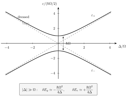
The detuned rotating-wave Hamiltonian converts the bare crossing into an avoided crossing of gap $\hbar\Omega$. Far from resonance, each bare-connected branch is displaced by a second-order amount proportional to $\Omega^2/\Delta$. At resonance the bare-state shift language fails and the appropriate description is dressed-state splitting.

Exact Dressed-Branch Shifts

Following the ground-like and excited-like branches

At $\Omega=0$, the rotating-frame bare energies are

$$\varepsilon_e^{(0)} = + \frac{\hbar\Delta}{2}, \qquad \varepsilon_g^{(0)} = - \frac{\hbar\Delta}{2}.$$

When $\Delta>0$, $|g\rangle$ connects to the lower dressed branch. When $\Delta<0$, it connects to the upper branch. The ground-connected quasienergy can therefore be written

$$\varepsilon_{g,\mathrm{ad}} = - \operatorname{sgn}(\Delta) \frac{\hbar\Omega_R}{2},$$

and the excited-connected branch has the opposite sign.

Subtracting the corresponding bare quasienergies gives

$$\begin{aligned} \delta E_g &= - \operatorname{sgn}(\Delta) \frac{\hbar}{2} \left( \Omega_R-|\Delta| \right), \\ \delta E_e &= + \operatorname{sgn}(\Delta) \frac{\hbar}{2} \left( \Omega_R-|\Delta| \right). \end{aligned}$$

These expressions remain exact within the constant-drive two-level RWA for $\Delta\ne0$. They also make the sign reversal across resonance explicit.

No bare-state shift at exact resonance

At

$$\Delta=0,$$

the eigenstates are equal superpositions of $|g\rangle$ and $|e\rangle$, with separation

$$\varepsilon_+-\varepsilon_- = \hbar\Omega.$$

Neither branch is uniquely “the shifted ground state” or “the shifted excited state.” A perturbative formula proportional to $1/\Delta$ diverges because its bare-state labeling has lost validity, not because an observable energy becomes infinite.

Near resonance, one should use the dressed-state description or solve the open-system response. A separate weak probe can resolve an Autler–Townes doublet; a single driven transition can show Rabi oscillations and power broadening.

Far-Detuned Level Shifts

Suppose

$$|\Omega| \ll |\Delta|.$$

Then

$$\begin{aligned} \Omega_R &= |\Delta| \sqrt{ 1+ \frac{\Omega^2}{\Delta^2} } \\ &= |\Delta| + \frac{\Omega^2}{2|\Delta|} - \frac{\Omega^4}{8|\Delta|^3} + O \left( \frac{\Omega^6}{|\Delta|^5} \right). \end{aligned}$$

Therefore,

$$\delta E_g = - \frac{ \hbar\Omega^2 }{ 4\Delta } + \frac{ \hbar\Omega^4 }{ 16\Delta^3 } + O \left( \frac{\hbar\Omega^6}{\Delta^5} \right),$$

and

$$\delta E_e = + \frac{ \hbar\Omega^2 }{ 4\Delta } - \frac{ \hbar\Omega^4 }{ 16\Delta^3 } + O \left( \frac{\hbar\Omega^6}{\Delta^5} \right).$$

The leading two-level differential shift is

$$\delta\omega_{eg} = \frac{ \delta E_e-\delta E_g }{ \hbar } \simeq \frac{\Omega^2}{2\Delta}.$$

This is a shift of the transition frequency. A common shift of both levels would not appear in spectroscopy, although it could still affect center-of-mass motion if it varies in space.

Sign audit

Under the convention $\Delta=\omega_0-\omega_L$:

• red detuning has $\Delta>0$ and gives $\delta E_g<0$;
• blue detuning has $\Delta<0$ and gives $\delta E_g>0$;
• the excited-state shift has the opposite sign in the closed two-level model;
• changing to the alternative convention $\Delta_L=\omega_L-\omega_0$ reverses every displayed denominator.

The reliable procedure is to derive the shift from the declared Hamiltonian, not to memorize “red is negative” without recording the detuning definition.

Error of the quadratic approximation

Define

$$\eta = \frac{|\Omega|}{|\Delta|}.$$

The exact magnitude of the ground-branch shift is

$$|\delta E_g|_{\mathrm{exact}} = \frac{ \hbar|\Delta| }{ 2 } \left( \sqrt{1+\eta^2}-1 \right).$$

The leading approximation is

$$|\delta E_g|_{(2)} = \frac{ \hbar|\Delta|\eta^2 }{ 4 }.$$

Their relative difference begins as

$$\frac{ |\delta E_g|_{(2)} - |\delta E_g|_{\mathrm{exact}} }{ |\delta E_g|_{\mathrm{exact}} } = \frac{\eta^2}{4} + O(\eta^4).$$

Thus a small excited-state population is not the only accuracy criterion. Long coherent evolution can resolve a fourth-order phase correction even when $\eta^2\ll1$.

Virtual Admixture and Phase

What virtual excitation means

For $|\Omega/\Delta|\ll1$, the ground-connected dressed state contains an excited-state amplitude of order

$$c_e \sim - \frac{\Omega}{2\Delta}.$$

Its excited-state probability is therefore

$$P_e^{(\mathrm{adm})} \sim \frac{\Omega^2}{4\Delta^2}.$$

The word virtual means that the excited component is part of an off-resonant dressed eigenstate rather than an independently populated, energy-conserving final state. It does not mean that energy conservation may be violated for a time fixed by an uncertainty relation.

The energy shift is first order in the small admixture amplitude times the coupling, hence second order in $\Omega$:

$$\delta E \sim \hbar\Omega \left( \frac{\Omega}{\Delta} \right).$$

Phase accumulation without population transfer

If the field envelope varies in time while the system follows one dressed branch,

$$|\psi_n(T)\rangle \sim \exp \left[ - \frac{i}{\hbar} \int_0^T \delta E_n(t)\,dt \right] |n\rangle,$$

apart from the bare dynamical phase and any geometric contribution.

For a far-detuned ground state,

$$\begin{aligned} \phi_g^{(\mathrm{LS})} &= - \frac1\hbar \int_0^T \delta E_g(t)\,dt \\ &\simeq \int_0^T \frac{ |\Omega(t)|^2 }{ 4\Delta(t) } dt. \end{aligned}$$

A tiny instantaneous shift can therefore create a large coherent phase over a long interrogation.

Adiabatic turn-on condition

Introduce a mixing angle through

$$\tan2\theta = \frac{\Omega}{\Delta}.$$

Then

$$\dot\theta = \frac{ \Delta\dot\Omega-\Omega\dot\Delta }{ 2 \left( \Delta^2+\Omega^2 \right) }.$$

Following one dressed branch requires approximately

$$|\dot\theta| \ll \Omega_R.$$

If a pulse switches too abruptly, it can leave coherent population transfer or ringing in addition to the intended phase. “Far detuned” does not by itself guarantee adiabatic turn-on.

Beyond the Rotating-Wave Approximation

Rotating and counter-rotating denominators

Second-order Floquet perturbation theory for a real cosine field gives, for the two-level ground state,

$$\begin{aligned} \delta E_g \simeq - \frac{ \hbar\Omega^2 }{ 4 } \left[ \frac{1}{ \omega_0-\omega_L } + \frac{1}{ \omega_0+\omega_L } \right]. \end{aligned}$$

The excited-state shift has the opposite sign within this ideal model. The first denominator is the co-rotating contribution retained by the RWA. The second is the leading counter-rotating contribution.

Near resonance,

$$|\omega_0-\omega_L| \ll \omega_0+\omega_L,$$

so the RWA term dominates the off-resonant shift. Precision spectroscopy can still resolve the smaller correction.

Bloch–Siegert connection

The counter-rotating contribution changes the transition frequency by

$$\delta\omega_{\mathrm{BS}} \simeq \frac{ \Omega^2 }{ 2 \left( \omega_0+\omega_L \right) }.$$

Near $\omega_L\simeq\omega_0$,

$$\delta\omega_{\mathrm{BS}} \simeq \frac{\Omega^2}{4\omega_0}.$$

This coefficient follows the present lab-frame convention, in which the RWA Hamiltonian has transverse term $\hbar\Omega\sigma_x/2$. Other definitions of drive amplitude move factors of two. The Hamiltonian must accompany any quoted Bloch–Siegert formula.

Multilevel systems

For a real atom or molecule, every dipole-coupled intermediate state brings both rotating and counter-rotating denominators. Contributions can have different signs and can cancel. A two-level estimate is reliable only when one transition dominates both the shift and the relevant scattering error.

Dynamic-Polarizability Dictionary

For a nondegenerate state $|n\rangle$ in a weak monochromatic field with peak amplitude $E_0$, define the real dispersive light shift by

$$\delta E_n = - \frac14 \operatorname{Re} \left[ \alpha_n(\omega_L) \right] E_0^2.$$

Using

$$I = \frac12\epsilon_0cE_0^2,$$

the same relation is

$$\delta E_n = - \frac{ \operatorname{Re}\alpha_n(\omega_L) }{ 2\epsilon_0c } I.$$

The dynamic polarizability packages the complete sum over intermediate states, polarizations, and both frequency denominators. Its imaginary part describes dissipative response under a declared Fourier and linewidth convention.

For the ideal two-level ground state,

$$\alpha_g(\omega) = \frac{ 2\omega_0|d_{eg}|^2 }{ \hbar \left( \omega_0^2-\omega^2 \right) }.$$

Substitution into $-\alpha E_0^2/4$ reproduces the rotating and counter-rotating shift above.

Peak, RMS, and static fields

Because

$$E_{\mathrm{rms}} = \frac{E_0}{\sqrt2},$$

one may also write

$$\delta E_n = - \frac12 \operatorname{Re}\alpha_n(\omega) E_{\mathrm{rms}}^2.$$

For a truly static field of magnitude $E_{\mathrm{dc}}$, the quadratic shift is

$$\delta E_n^{\mathrm{dc}} = - \frac12 \alpha_n(0) E_{\mathrm{dc}}^2.$$

The AC formula with a fixed peak amplitude contains the additional cycle-average factor $1/2$. Taking $\omega\to0$ after averaging over an ever-longer cycle is not the same experimental operation as applying a constant field $E_0$.

Scalar, Vector, and Tensor Light Shifts

For angular-momentum manifolds, the response is generally not one scalar number. It decomposes into irreducible contributions.

Scalar part

The scalar shift:

• is independent of magnetic sublevel within the ideal manifold;
• follows the local intensity;
• produces a common trapping potential for states with the same scalar polarizability.

It can still be differential between two clock or qubit states.

Vector part

The vector shift:

• depends on optical helicity;
• changes sign with magnetic quantum number or reversed circular polarization;
• behaves like a light-induced effective magnetic field;
• vanishes for ideal linear polarization in the simplest geometry.

Residual ellipticity can therefore convert polarization drift into a frequency shift.

Tensor part

The tensor shift:

• depends on polarization alignment relative to the quantization axis;
• produces an even-in-$m$ splitting pattern;
• requires sufficient angular momentum at the relevant electronic or hyperfine level;
• can survive even when vector shifts are canceled by averaging opposite magnetic substates.

Exact normalizations of scalar, vector, and tensor polarizabilities differ among references. A coefficient is incomplete unless the angular-momentum, polarization, and reduced-matrix-element conventions are supplied.

Practical symmetry reversals

Useful diagnostics include:

• reverse helicity to isolate vector contributions;
• compare $+m$ and $-m$ states;
• rotate the quantization axis relative to linear polarization;
• vary intensity to separate leading $I$ and hyperpolarizability $I^2$ terms;
• vary optical frequency to map dispersive sign changes.

These reversals separate irreducible responses more reliably than a single-intensity measurement.

Shift and Photon-Scattering Tradeoff

A far-detuned field does not make the excited-state admixture exactly zero. If the excited state decays at population rate $\Gamma$, the admixture produces the approximate scattering rate

$$\Gamma_{\mathrm{sc}} \simeq \Gamma \frac{ \Omega^2 }{ 4\Delta^2 }$$

for a weak, isolated two-level transition.

The ground-state light-shift magnitude is

$$|U_g| \simeq \frac{ \hbar\Omega^2 }{ 4|\Delta| }.$$

Their ratio is

$$\frac{ \hbar\Gamma_{\mathrm{sc}} }{ |U_g| } \simeq \frac{\Gamma}{|\Delta|}.$$

At fixed trap depth or phase rate, larger detuning reduces scattering in this ideal model, but maintaining the same shift then requires intensity proportional to $|\Delta|$. Available power, nearby transitions, photoionization, technical noise, and multilevel interference eventually limit this simple scaling.

Coherent and incoherent errors scale differently

For one dominant line:

$$|\delta E| \propto \frac{I}{|\Delta|}, \qquad \Gamma_{\mathrm{sc}} \propto \frac{I}{\Delta^2}.$$

Thus:

• light-shift phase is first order in $1/\Delta$;
• scattering probability is second order in $1/\Delta$;
• increasing detuning at fixed intensity reduces both, but the scattering falls faster;
• increasing intensity to hold the phase fixed leaves a residual scattering cost proportional to $1/|\Delta|$.

Real multilevel systems can violate the one-line ratio because amplitudes and decay branches combine differently.

Optical Dipole Potentials

If the field intensity varies slowly across the internal wavefunction, the position-dependent light shift becomes a center-of-mass potential:

$$U_n(\mathbf r) = - \frac{ \operatorname{Re}\alpha_n(\omega_L) }{ 2\epsilon_0c } I(\mathbf r).$$

The conservative dipole force is

$$\mathbf F_n(\mathbf r) = - \boldsymbol\nabla U_n(\mathbf r).$$

In the dominant two-level ground-state limit,

$$U_g(\mathbf r) \simeq - \frac{ \hbar|\Omega(\mathbf r)|^2 }{ 4\Delta }.$$

With this page’s detuning convention:

• a red-detuned field has $\Delta>0$ and attracts the ground state toward high intensity;
• a blue-detuned field has $\Delta<0$ and repels it toward low intensity.

For a multilevel atom, the sign of the full polarizability, not the nearest line alone, decides where the atom is trapped.

Conservative-potential conditions

Treating $U_n(\mathbf r)$ as a scalar mechanical potential requires:

1. internal dressed-state following is adiabatic during motion;
2. photon scattering is slow on the mechanical time scale;
3. polarization gradients and vector/tensor forces are controlled;
4. the field varies slowly over the internal size of the particle;
5. nonadiabatic transitions at avoided crossings are negligible.

If the local dressed eigenvectors vary in space, motion can also acquire geometric vector and scalar potentials. Those effects are not contained in the simple gradient of one scalar $\alpha I$.

Trap depth is not the whole error model

Two traps with the same depth can have different:

• scattering and recoil-heating rates;
• differential shifts between internal states;
• sensitivity to intensity noise;
• polarization gradients;
• anharmonicity and tunneling;
• sensitivity to nearby molecular or atomic resonances.

The shift and the loss rate must be calculated from the same declared internal model.

Differential Shifts in Spectroscopy

For a transition between states $|a\rangle$ and $|b\rangle$,

$$\delta\omega_{ba} = \frac{ \delta E_b-\delta E_a }{ \hbar }.$$

In the scalar polarizability limit,

$$\delta\nu_{ba} = - \frac{ \Delta\alpha_{ba}(\omega_L) }{ 2h\epsilon_0c } I,$$

where

$$\Delta\alpha_{ba} = \alpha_b-\alpha_a.$$

A large common light shift can coexist with a small transition shift. Conversely, a weakly trapped state pair can have a large differential shift.

Spatially inhomogeneous light

If particles sample different intensities,

$$\delta\omega_{ba} = \delta\omega_{ba} \left[ I(\mathbf r) \right],$$

then one nominal transition becomes a distribution of local frequencies. The result can be:

• an inhomogeneously broadened line;
• an asymmetric line if density and intensity are correlated;
• dephasing from motion through the gradient;
• a temperature-dependent fitted center;
• sidebands when motion is quantized and resolved.

Replacing $I(\mathbf r)$ by one mean value can bias both line center and linewidth.

Probe light versus trapping light

A trapping field may be present continuously, while a probe field exists only during interrogation pulses. Their shifts enter differently:

• a continuous trap changes the energy splitting throughout free evolution;
• a pulsed probe can add phase only during the pulses;
• Ramsey and composite-pulse sequences convert that phase into a lock-point shift in a protocol-dependent way;
• switching transients can produce chirps and nonadiabatic excitation.

A clock correction therefore needs the complete timing sequence, not only a static value of $\delta\nu/I$.

Clock-Systematic Connection

Magic operation

A leading electric-dipole magic frequency satisfies

$$\Delta\alpha_{ba}(\omega_{\mathrm m}) = 0$$

for a specified pair of states, polarization, magnetic sublevel, and geometry. The common optical potential can remain nonzero, allowing confinement with a canceled leading differential shift.

“Magic” does not mean field free. Residual terms can include:

• vector and tensor light shifts;
• electric-quadrupole and magnetic-dipole response;
• hyperpolarizability proportional to $I^2$;
• multiphoton resonances;
• motional sampling and lattice anharmonicity;
• imperfect polarization and magnetic-field alignment.

Probe-induced shifts

The clock probe can couple each clock state to off-resonant spectator states. Its differential shift often scales as

$$\delta\nu_{\mathrm{probe}} \propto I_{\mathrm{probe}}$$

in the weak-field regime. Useful controls include:

1. interleave measurements at several probe intensities;
2. extrapolate to zero intensity only after testing linearity;
3. apply a calibrated frequency step during pulses;
4. reverse polarization or magnetic sublevel where symmetry permits;
5. use hyper-Ramsey or autobalanced protocols when pulse-only shifts dominate;
6. monitor pulse transients and optical phase chirps independently.

Composite interrogation can suppress sensitivity to a modeled shift, but it does not remove the need to validate the model and bound residual imperfections.

Light Shifts in Raman and Effective Couplings

In a detuned three-level Raman system, eliminating the intermediate state generates both:

• an off-diagonal two-photon coupling of order $\Omega_1^*\Omega_2/\Delta$;
• diagonal light shifts of order $|\Omega_1|^2/\Delta$ and $|\Omega_2|^2/\Delta$.

They occur at the same perturbative order. Keeping the effective Raman coupling while dropping both diagonal shifts is generally inconsistent.

The Raman resonance condition is displaced by the differential light shift:

$$\delta_{\mathrm{2ph,eff}} = \delta_{\mathrm{2ph}} + \frac{ \delta E_2-\delta E_1 }{ \hbar }.$$

Balancing intensities can cancel a differential shift in one idealized model, but unequal detunings, hyperfine pathways, polarization impurity, spontaneous scattering, and spatial mode mismatch can leave a residual.

Experimental Forward Models

Intensity scan

In the perturbative scalar regime,

$$\nu_{\mathrm{obs}}(I) = \nu_0+\kappa I,$$

with

$$\kappa = - \frac{ \Delta\alpha }{ 2h\epsilon_0c }.$$

A reliable extraction should test:

• linearity over the fitted intensity range;
• calibration of intensity at the particle rather than at a remote monitor;
• spatial averaging and temperature dependence;
• polarization and magnetic-field stability;
• correlations between intensity and line-shape asymmetry.

Curvature can indicate hyperpolarizability, saturation, changing spatial sampling, or a drifting population distribution.

Detuning scan

For one dominant spectator line,

$$\delta E \propto \frac{1}{\Delta},$$

so the shift changes sign across resonance. Close enough to resonance, however, scattering and dressed-state splitting invalidate the purely dispersive fit. Excluding the central region is a physical model choice, not merely a plotting preference.

Pulse-area scan

If the same field drives the intended transition and couples off-resonantly to spectators, changing pulse area by changing intensity also changes the light shift. A Rabi-frequency calibration and a frequency calibration are then coupled. Jointly fitting power-dependent chevrons or Ramsey phases is safer than fixing a zero-power resonance center.

Pump-on and pump-off references

Measure the unperturbed frequency by interleaving field conditions faster than relevant drifts. A useful cycle may compare:

• nominal intensity;
• a lower intensity;
• reversed helicity;
• opposite magnetic sublevels;
• shifted optical frequency;
• dark or zero-intensity reference shots.

The interleaving pattern should distinguish a physical light shift from laser-frequency drift, magnetic drift, and servo error.

A Reliable Calculation Workflow

1. Declare states and conventions. Record the ordered basis, detuning sign, peak or RMS field, and Rabi-frequency definition.
2. Inventory coupled levels. Apply selection rules and include every nearby state relevant at the target accuracy.
3. Choose a regime. Use exact dressed eigenvalues near resonance and a perturbative polarizability only where denominators dominate couplings and linewidths.
4. Retain counter-rotating terms when required. Compare the target uncertainty with the Bloch–Siegert and remote-line scales.
5. Compute each level shift. A measured transition uses their difference, not either shift alone.
6. Add dissipation consistently. Use the same matrix elements and detunings for scattering and dispersive response.
7. Resolve angular structure. Include scalar, vector, tensor, and polarization geometry at the required level.
8. Map the spatial field. Average over particle position, motion, and internal-state distribution.
9. Model the pulse sequence. A shift present only during pulses enters Ramsey and composite spectroscopy differently from a continuous shift.
10. Test reversals and scaling. Detuning sign, intensity, helicity, magnetic sublevel, and timing provide independent diagnostics.

Common Mistakes

Mixing detuning conventions

With $\Delta=\omega_0-\omega_L$, red detuning is positive and $\delta E_g=-\hbar\Omega^2/(4\Delta)$. References using $\omega_L-\omega_0$ display the opposite sign in the denominator.

Losing the field-amplitude factor

The shift is $-\alpha E_0^2/4$ for a sinusoid with peak amplitude $E_0$, but $-\alpha E_{\mathrm{rms}}^2/2$ in RMS notation.

Extending the inverse-detuning formula through resonance

At $\Delta=0$, the correct RWA result is a dressed splitting $\hbar\Omega$, not an infinite level shift.

Calling virtual population exactly zero

The admixture is small, of order $\Omega/(2\Delta)$, but its square produces spontaneous scattering when the coupled state decays.

Dropping the counter-rotating term at precision level

The RWA can be excellent for population dynamics while its Bloch–Siegert correction remains resolvable in a frequency measurement.

Using one level shift for a transition

Spectroscopy measures

$$\delta E_b-\delta E_a.$$

Common-mode shifts cancel from the transition frequency.

Treating all light shifts as scalar

Ellipticity, quantization-axis geometry, and magnetic sublevel can activate vector and tensor terms.

Equating a conservative potential with zero scattering

A real light shift and an imaginary dissipative response are two parts of the same driven susceptibility. Far detuning suppresses scattering but does not erase it.

Assuming a two-level atom because one line is nearest

Remote levels may contribute little population yet materially change a precision shift through coherent sums. Near cancellations are especially sensitive to omitted terms.

Dropping Raman light shifts

The diagonal shifts and off-diagonal effective coupling arise at the same order in adiabatic elimination.

Calling a magic wavelength universally magic

The cancellation belongs to specified states, polarization, geometry, and perturbative order. Higher-order and multipolar shifts can remain.

Key Results

1. The exact RWA quasienergies are $\varepsilon_\pm=\pm\hbar\sqrt{\Delta^2+\Omega^2}/2$.
2. Far from resonance, $\delta E_g=-\hbar\Omega^2/(4\Delta)$ and $\delta E_e=+\hbar\Omega^2/(4\Delta)$.
3. The bare-state shift picture fails at resonance, where the dressed gap is $\hbar\Omega$.
4. A smooth off-resonant pulse can accumulate phase with little final population transfer.
5. Counter-rotating terms produce the Bloch–Siegert correction.
6. In the weak scalar regime, $\delta E=-\operatorname{Re}\alpha(\omega)I/(2\epsilon_0c)$.
7. For one far-detuned lossy line, $\hbar\Gamma_{\mathrm{sc}}/|U|\simeq\Gamma/|\Delta|$.
8. Optical trapping uses a spatially varying level shift; clocks measure a differential shift and require protocol-aware calibration.

Further Connections

• Stark Effect in Atoms compares DC and AC response and develops atom-specific tensor structure.
• Dynamic Polarizability develops the complete causal response tensor, spectral sums, tune-out zeros, magic crossings, and uncertainty propagation.
• Optical Dipole Traps turns spatially varying light shifts into calibrated trap depths, normal-mode frequencies, and heating budgets.
• Optical Lattices uses interference to make periodic light shifts and develops recoil, band, loading, and lattice-model calibration.
• Optical Clocks applies differential light shifts to probe, lattice, blackbody, and operational magic-point evaluations.
• Rabi Oscillations explains the coherent population dynamics that replaces perturbative shift language near resonance.
• Dressed States develops exact branch composition, avoided-crossing identity, adiabatic preparation, and atom–photon doublets.
• Autler–Townes Splitting develops the near-resonant weak-probe spectrum and its resolvability criteria.
• Optical Bloch Equations provides the dissipative line shape, saturation parameter, and scattering rate beyond the far-detuned estimate.
• Radiation Pressure separates dissipative momentum transfer and recoil diffusion from the conservative force generated by a light-shift gradient.
• Adiabatic Elimination derives Raman light shifts and effective two-photon couplings together.
• Ramsey Interferometry shows how pulse-dependent phases become fringe and clock-frequency shifts.
• Precision Spectroscopy develops interleaved measurements, systematic corrections, and uncertainty budgets.

References

1. S. H. Autler and C. H. Townes, “Stark Effect in Rapidly Varying Fields,” Physical Review 100, 703–722 (1955).
2. F. Bloch and A. Siegert, “Magnetic Resonance for Nonrotating Fields,” Physical Review 57, 522–527 (1940).
3. J. Dalibard and C. Cohen-Tannoudji, “Dressed-Atom Approach to Atomic Motion in Laser Light: The Dipole Force Revisited,” Journal of the Optical Society of America B 2, 1707–1720 (1985).
4. R. Grimm, M. Weidemüller, and Y. B. Ovchinnikov, “Optical Dipole Traps for Neutral Atoms,” Advances in Atomic, Molecular, and Optical Physics 42, 95–170 (2000).
5. H. Katori, M. Takamoto, V. G. Pal’chikov, and V. D. Ovsiannikov, “Ultrastable Optical Clock with Neutral Atoms in an Engineered Light Shift Trap,” Physical Review Letters 91, 173005 (2003).
6. A. D. Ludlow, M. M. Boyd, J. Ye, E. Peik, and P. O. Schmidt, “Optical Atomic Clocks,” Reviews of Modern Physics 87, 637–701 (2015).
7. V. I. Yudin et al., “Hyper-Ramsey Spectroscopy of Optical Clock Transitions,” Physical Review A 82, 011804(R) (2010).
8. C. Cohen-Tannoudji, J. Dupont-Roc, and G. Grynberg, Atom–Photon Interactions: Basic Processes and Applications (Wiley, 1992).
9. B. W. Shore, The Theory of Coherent Atomic Excitation (Wiley, 1990).

Exercises

1. Exact branches and the far-detuned limit

Diagonalize

$$H = \frac{\hbar}{2} \begin{pmatrix} \Delta & \Omega \\ \Omega & -\Delta \end{pmatrix}$$

and derive the leading shifts of the bare-connected states for both signs of $\Delta$.

Solution

The characteristic equation is

$$\varepsilon^2 - \frac{\hbar^2}{4} \left( \Delta^2+\Omega^2 \right) = 0.$$

Therefore,

$$\varepsilon_\pm = \pm \frac{\hbar}{2} \sqrt{ \Delta^2+\Omega^2 }.$$

For $\Delta>0$, the ground state follows $\varepsilon_-$ and the excited state follows $\varepsilon_+$. Expanding gives

$$\begin{aligned} \varepsilon_- &= - \frac{\hbar\Delta}{2} - \frac{\hbar\Omega^2}{4\Delta} + O(\Omega^4/\Delta^3), \\ \varepsilon_+ &= + \frac{\hbar\Delta}{2} + \frac{\hbar\Omega^2}{4\Delta} + O(\Omega^4/\Delta^3). \end{aligned}$$

For $\Delta<0$, the ground state follows $\varepsilon_+$ and the excited state follows $\varepsilon_-$. The same compact formulas result:

$$\delta E_g = - \frac{\hbar\Omega^2}{4\Delta}, \qquad \delta E_e = + \frac{\hbar\Omega^2}{4\Delta}.$$

Their signs reverse because the denominator changes sign.

2. Check the expansion error

Let

$$\eta = \frac{|\Omega|}{|\Delta|}.$$

Evaluate the exact and second-order ground-shift magnitudes in units of $\hbar|\Delta|$ for $\eta=0.20$. Find their relative difference.

Solution

The exact dimensionless magnitude is

$$\frac{ |\delta E_g|_{\mathrm{exact}} }{ \hbar|\Delta| } = \frac12 \left( \sqrt{1+\eta^2}-1 \right).$$

At $\eta=0.20$,

$$\sqrt{1+\eta^2} = \sqrt{1.04} \simeq 1.0198039,$$

so

$$\frac{ |\delta E_g|_{\mathrm{exact}} }{ \hbar|\Delta| } \simeq 0.00990195.$$

Second order gives

$$\frac{ |\delta E_g|_{(2)} }{ \hbar|\Delta| } = \frac{\eta^2}{4} = 0.0100000.$$

The relative overestimate is

$$\begin{aligned} \epsilon_{\mathrm{rel}} &= \frac{ 0.0100000-0.00990195 }{ 0.00990195 } \\ &\simeq 9.90\times10^{-3}. \end{aligned}$$

Thus the second-order result is high by about $0.99\%$.

3. Light shift and virtual population

A two-level atom has

$$\begin{aligned} \Delta &= 2\pi\times1.00\ \mathrm{GHz}, \\ \Omega &= 2\pi\times20.0\ \mathrm{MHz}. \end{aligned}$$

Estimate:

1. the ground-state light shift in ordinary frequency;
2. the excited-state admixture probability;
3. the scattering rate if $\Gamma=2\pi\times6.00\ \mathrm{MHz}$.

Solution

The angular-frequency light shift is

$$\frac{\delta E_g}{\hbar} \simeq - \frac{\Omega^2}{4\Delta}.$$

Dividing by $2\pi$ and using ordinary-frequency values consistently,

$$\frac{\delta E_g}{h} \simeq - \frac{ (20.0\ \mathrm{MHz})^2 }{ 4(1000\ \mathrm{MHz}) } = -0.100\ \mathrm{MHz}.$$

Thus

$$\frac{\delta E_g}{h} \simeq -100\ \mathrm{kHz}.$$

The admixture probability is

$$P_e^{(\mathrm{adm})} \simeq \frac14 \left( \frac{20.0}{1000} \right)^2 = 1.00\times10^{-4}.$$

The scattering rate is

$$\Gamma_{\mathrm{sc}} \simeq \Gamma P_e^{(\mathrm{adm})}.$$

Therefore,

$$\Gamma_{\mathrm{sc}} \simeq 2\pi\times600\ \mathrm{Hz},$$

or about

$$3.77\times10^3\ \mathrm{s^{-1}}.$$

4. Phase from a Gaussian pulse

A far-detuned field has constant detuning $\Delta$ and Rabi envelope

$$\Omega(t) = \Omega_0 e^{-t^2/(2\tau^2)}.$$

Find the light-shift phase accumulated by the ground state from $t=-\infty$ to $+\infty$.

Solution

The ground-state phase is

$$\phi_g^{(\mathrm{LS})} \simeq \int_{-\infty}^{\infty} \frac{ |\Omega(t)|^2 }{ 4\Delta } dt.$$

Because

$$|\Omega(t)|^2 = \Omega_0^2e^{-t^2/\tau^2},$$

and

$$\int_{-\infty}^{\infty} e^{-t^2/\tau^2}\,dt = \sqrt\pi\,\tau,$$

the result is

$$\phi_g^{(\mathrm{LS})} = \frac{ \sqrt\pi\, \Omega_0^2\tau }{ 4\Delta }.$$

Its sign follows the sign of $\Delta$. The result assumes adiabatic following and negligible scattering.

5. Counter-rotating correction

Let

$$\omega_L \simeq \omega_0 = 2\pi\times5.00\ \mathrm{GHz},$$

and

$$\Omega = 2\pi\times50.0\ \mathrm{MHz}.$$

Estimate the Bloch–Siegert shift in ordinary frequency using this page’s Hamiltonian convention.

Solution

Near resonance,

$$\delta\omega_{\mathrm{BS}} \simeq \frac{\Omega^2}{4\omega_0}.$$

Because every angular frequency contains one common factor $2\pi$,

$$\frac{ \delta\omega_{\mathrm{BS}} }{ 2\pi } = \frac{ (50.0\ \mathrm{MHz})^2 }{ 4(5000\ \mathrm{MHz}) }.$$

Hence

$$\frac{ \delta\omega_{\mathrm{BS}} }{ 2\pi } = 0.125\ \mathrm{MHz} = 125\ \mathrm{kHz}.$$

The correction is small compared with the carrier frequency but can be large compared with a precision spectroscopic uncertainty.

6. Optical potential and scattering budget

A ground-state optical trap has depth

$$\frac{|U|}{h} = 1.00\ \mathrm{MHz}.$$

The dominant optical line has

$$\begin{aligned} \Gamma &= 2\pi\times6.00\ \mathrm{MHz}, \\ |\Delta| &= 2\pi\times100\ \mathrm{THz}. \end{aligned}$$

Use the two-level far-detuned ratio to estimate the scattering rate.

Solution

Use

$$\Gamma_{\mathrm{sc}} \simeq \frac{\Gamma}{|\Delta|} \frac{|U|}{\hbar}.$$

The frequency ratio is

$$\frac{\Gamma}{|\Delta|} = \frac{ 6.00\times10^6 }{ 1.00\times10^{14} } = 6.00\times10^{-8}.$$

Also,

$$\frac{|U|}{\hbar} = 2\pi\times1.00\times10^6\ \mathrm{s^{-1}}.$$

Therefore,

$$\begin{aligned} \Gamma_{\mathrm{sc}} &\simeq (6.00\times10^{-8}) (2\pi\times10^6) \\ &\simeq 0.377\ \mathrm{s^{-1}}. \end{aligned}$$

The estimated mean scattering time is about $2.65\ \mathrm s$. A real atom requires a multilevel calculation before treating this number as predictive.

7. Differential clock shift

At one lattice frequency,

$$\frac{ \Delta\alpha }{ h } = 2.00\times10^{-4} \frac{ \mathrm{Hz\,m^2} }{ \mathrm{V^2} }.$$

The peak electric-field amplitude is

$$E_0 = 1.00\times10^4\ \mathrm{V/m}.$$

Find the scalar differential clock shift. What happens to the leading result at a magic frequency?

Solution

With a peak field,

$$\delta\nu = - \frac14 \frac{\Delta\alpha}{h} E_0^2.$$

The product is

$$\frac{\Delta\alpha}{h}E_0^2 = 2.00\times10^4\ \mathrm{Hz}.$$

Therefore,

$$\begin{aligned} \delta\nu &= - \frac14 \left( 2.00\times10^4\ \mathrm{Hz} \right) \\ &= -5.00\times10^3\ \mathrm{Hz}. \end{aligned}$$

At a leading-order electric-dipole magic frequency,

$$\Delta\alpha(\omega_{\mathrm m}) = 0,$$

so this term vanishes. Vector, tensor, multipolar, hyperpolarizability, and motional corrections may remain.

8. Diagnose light-shift symmetry

An experiment measures a transition at magnetic substates $+m$ and $-m$ with right- and left-circular polarization. Propose combinations of the four frequencies that isolate an $m$-odd vector light shift from an $m$-even scalar-plus-tensor shift.

Solution

Write the frequency schematically as

$$\nu(m,\xi) = \nu_{\mathrm{even}}(m^2) + \xi m\,\nu_{\mathrm v},$$

where $\xi=+1$ and $-1$ label opposite helicities.

At fixed helicity, the $m$-odd combination is

$$\frac{ \nu(+m,\xi)-\nu(-m,\xi) }{ 2 } = \xi m\,\nu_{\mathrm v}.$$

Equivalently, at fixed $m$,

$$\frac{ \nu(m,+)-\nu(m,-) }{ 2 } = m\,\nu_{\mathrm v}.$$

A useful normalized $m$-reversal difference at each helicity is

$$D_\xi = \frac{ \nu(+m,\xi)-\nu(-m,\xi) }{ 2m } = \xi\nu_{\mathrm v}.$$

A robust vector estimator is therefore

$$\nu_{\mathrm v}^{(\mathrm{est})} = \frac{ D_+-D_- }{ 2 }.$$

For the even response, define

$$\overline\nu_\xi = \frac{ \nu(+m,\xi)+\nu(-m,\xi) }{ 2 }.$$

The fully even average is

$$\frac{ \overline\nu_+ + \overline\nu_- }{ 2 }.$$

removes the ideal vector term and retains the scalar contribution plus any $m$-even tensor shift. Additional orientations or magnetic-sublevel values are needed to separate scalar from tensor response.