Precision Spectroscopy

Precision spectroscopy estimates an unperturbed quantum transition frequency, frequency ratio, or other spectral parameter together with a traceable uncertainty. The goal is not merely to display many digits. It is to establish which physical quantity those digits represent, how the apparatus perturbed it, how the corrections were evaluated, and which inference remains after statistical and systematic effects are propagated.

For two stationary states of the isolated model,

$$\nu_0=\frac{E_b-E_a}{h}.$$

A laboratory does not observe $\nu_0$ directly. It observes a response from atoms or molecules moving in finite fields, interrogated for finite time by an imperfect oscillator and detector. A minimal observation equation is

$$\nu_{\mathrm{obs}} = \nu_0 + \sum_k \Delta\nu_k + \epsilon,$$

where $\Delta\nu_k$ are modeled shifts and $\epsilon$ contains statistical fluctuations and any residual not represented explicitly. Precision spectroscopy is the discipline of making every term operational.

Canonical Scope

This page is the spectroscopy-centered gateway from a resolved line to frequency standards, fundamental constants, relativistic potential differences, and null searches. It owns the common inference chain and the distinction between an observed line center and an unperturbed transition.

Several ingredients have separate canonical homes:

• Line Shapes and Broadening owns homogeneous, inhomogeneous, Voigt, saturation, and line-pulling models.
• Hyperfine Structure, Zeeman Effect in Atoms, and Stark Effect in Atoms own the atom-specific Hamiltonians behind common shifts.
• Rabi and Ramsey Control owns the open-system pulse dynamics.
• Ramsey Interferometry owns the separated-pulse unitary, finite-pulse fringe shape, capture range, and clock error-signal construction summarized here.
• Multipole Expansion owns forbidden clock-line amplitudes, E2 and E3 rate scaling, and the distinction between transition and static quadrupole moments.
• Precision Measurement Applications owns the symmetry map for clocks, interferometers, magnetometry, and discrete-symmetry tests.
• Constants is the lookup home for current numerical values used in ordinary calculations.

The current SI definition is also a moving policy context. At this page’s review date, the second remains defined by assigning the exact value $9\,192\,631\,770\ \mathrm{Hz}$ to the unperturbed ground-state hyperfine transition frequency of $^{133}\mathrm{Cs}$. The BIPM also maintains optical and microwave secondary representations, while work toward a possible future redefinition is active. A secondary representation is not already a new definition.

Why Precision Spectra Matter

Spectral frequencies can be reproduced, counted, and compared with extraordinary fractional sensitivity. The same transition can play several roles:

Role	Measured object	Required interpretation
structure test	absolute frequency or interval	Hamiltonian, radiative and finite-size corrections
frequency reference	oscillator locked to a transition	realization, traceability, stability, uncertainty
constant determination	several observables in a global model	sensitivity coefficients and covariance
field sensor	differential shift	calibrated response to electric, magnetic, inertial, or gravitational fields
null test	frequency combination expected to vanish or remain fixed	symmetry, reversals, drift model, controls
new-physics search	anomalous time, space, isotope, or species dependence	signal template and Standard Model backgrounds

A line center is an estimator

A peak maximum, a fitted centroid, a Ramsey-fringe zero crossing, and a maximum-likelihood transition frequency are not automatically the same quantity. They coincide only under a stated response model. Asymmetry, unresolved neighbors, state-dependent loss, saturation, servo sampling, and detector nonlinearity can move an estimator even if no energy level has shifted.

Write the measured record as $D$ and the forward model as $p(D\mid\nu_0,\boldsymbol\theta)$, where $\boldsymbol\theta$ denotes nuisance parameters. Then a reported frequency is schematically

$$\widehat{\nu}_0 = \operatorname*{arg\,max}_{\nu_0} \mathcal L \left( \nu_0,\widehat{\boldsymbol\theta};D \right),$$

or the corresponding posterior summary in a Bayesian analysis. The fitting rule, prior information, excluded data, and model checks belong to the measurement result.

Resolution, precision, and uncertainty

These terms answer different questions:

Quantity	Question
resolution	Can nearby spectral features be distinguished?
repeatability	Do nominally identical measurements agree over a short interval?
stability	How does fractional frequency fluctuate with averaging time?
precision	How narrowly is a result distributed under the stated procedure?
systematic correction	What modeled displacement is applied to the result?
measurement uncertainty	What dispersion of values can reasonably be attributed to the measurand?
accuracy	Qualitative closeness to the quantity’s true value; not a substitute for an uncertainty statement

A narrow statistical interval does not guarantee small systematic uncertainty. Conversely, a large correction can be acceptable when the correction is well determined. What matters is the uncertainty remaining after the correction, not whether the correction happened to be numerically small.

Ratios are primary observables

An optical clock comparison naturally measures a dimensionless ratio,

$$R_{AB}=\frac{\nu_A}{\nu_B}.$$

Ratios avoid attaching significance to a conventional unit before the comparison is interpreted. They are also natural for tests of constants: different transitions have different dependence on $\alpha$, mass ratios, and nuclear parameters. A frequency ratio network can expose inconsistency through loop closure without requiring every edge to be measured against caesium at the same precision.

From Resonance to Claim

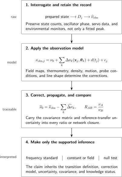
A reported precision frequency is the output of an observation model, not a label copied from a peak. Environmental monitors, correction coefficients, covariance, and reference traceability accompany the transition from $\nu_{\mathrm{obs}}$ to $\nu_0$ and then to a standard, constant, or null test.

For measurement cycle $j$, a useful model is

$$\begin{aligned} \nu_{\mathrm{obs},j} &= \nu_0 + \sum_k \Delta\nu_k \left( \mathbf x_j,\boldsymbol\theta_k \right) \\ &\quad + d(t_j) + \epsilon_j. \end{aligned}$$

Here $\mathbf x_j$ contains recorded conditions such as field, temperature, density, probe intensity, velocity, and gravitational potential; $\boldsymbol\theta_k$ contains calibrated response coefficients; and $d(t)$ represents oscillator or apparatus drift not removed by the interrogation scheme.

The corrected estimate is

$$\widehat{\nu}_0 = \widehat{\nu}_{\mathrm{obs}} - \sum_k \widehat{\Delta\nu}_k.$$

The signs must follow the declared observation equation. A table that lists a “correction” without saying whether it is added to the observed value or whether it denotes the physical shift is ambiguous.

Propagating uncertainty and covariance

Let the result be $y=f(\mathbf z)$, where $\mathbf z$ contains fitted line parameters, calibration inputs, and correction coefficients. To first order,

$$u_c^2(y) = \mathbf J \mathbf C_{\mathbf z} \mathbf J^{\mathsf T} + u_{\mathrm{model}}^2,$$

with

$$J_i = \frac{\partial f}{\partial z_i}.$$

$\mathbf C_{\mathbf z}$ is the input covariance matrix. The extra $u_{\mathrm{model}}$ symbolically represents model inadequacy that has been evaluated but is not captured by the local parameter covariance. It must not be used as a vague allowance for unknown unknowns.

For independent inputs, the familiar form is

$$u_c^2(y) = \sum_i \left( \frac{\partial f}{\partial z_i} \right)^2 u^2(z_i).$$

Independence must be justified. Two clocks in the same room may share blackbody sensors, magnetic references, links, local oscillators, or gravitational-potential models. Shared inputs create covariance that may cancel in one ratio and reinforce in another.

Traceability

Metrological traceability is a documented chain of calibrations linking a result to a reference, with uncertainty contributions stated along the chain. Traceability does not mean that every optical frequency is measured directly against caesium on every run. Optical ratios, frequency combs, satellite or fiber links, flywheel oscillators, and international time scales can form parts of the chain.

A complete result states:

1. the measurand and transition labels;
2. the interrogation and line-center estimator;
3. the correction convention;
4. the uncertainty model and covariance;
5. the reference and transfer chain;
6. the averaging interval and stability statistic;
7. the conditions under which the result is valid.

Frequency Standards

A frequency standard realizes a reproducible frequency. An atomic clock combines such a reference with an oscillator, interrogation, feedback, and a means to accumulate phase or time. The atoms do not emit a perfect sequence of ticks by themselves. A passive clock repeatedly compares an engineered oscillator with a quantum transition and steers the oscillator using an error signal.

The passive-clock loop

For a Ramsey sequence with free-evolution time $T$, a convenient idealized fringe is

$$P_e(\delta\nu) = \frac12 \left[ 1 + C \cos \left( 2\pi\delta\nu T+\phi \right) \right],$$

where

$$\delta\nu = \nu_{\mathrm{LO}}-\nu_0.$$

The local oscillator is sampled on opposite sides of the central fringe, or with opposite pulse phases, to form an error signal odd in $\delta\nu$. Feedback drives its long-term mean toward zero. In an actual clock, pulse errors, dead time, decoherence, servo gain, oscillator noise, and state detection modify this simple expression.

The central Ramsey feature has a width of order

$$\Delta\nu_{\mathrm{Ramsey}} \sim \frac{1}{2T}$$

for the ideal $\cos^2(\pi\delta\nu T)$ convention. This is interrogation resolution, not necessarily the natural linewidth.

The current SI second

The SI definition fixes

$$\Delta\nu_{\mathrm{Cs}} = 9\,192\,631\,770\ \mathrm{Hz}$$

exactly for the unperturbed ground-state hyperfine transition of $^{133}\mathrm{Cs}$. “Unperturbed” refers to an ideal reference condition. A caesium fountain realizes the definition by evaluating magnetic, blackbody, collisional, motional, microwave, and relativistic effects.

Optical transitions have much higher carrier frequencies and can offer larger quality factors and smaller evaluated fractional uncertainties. The BIPM’s recommended-frequency list includes optical secondary representations of the second. Their numerical values and uncertainties are periodically adjusted using absolute-frequency and optical-ratio data. This is a coordinated metrological network, not a contest in which one laboratory peak automatically replaces the SI definition.

Microwave and optical standards

Standard type	Typical transition	Principal strength	Characteristic challenge
thermal-beam microwave	ground-state hyperfine	robust historical realization	transit time and velocity distribution
fountain microwave	laser-cooled hyperfine	long ballistic interrogation	collisions, distributed cavity phase, microwave lensing
trapped-ion optical	weak electronic transition	excellent isolation and control	low signal rate, micromotion, logic/readout overhead
neutral-atom lattice optical	clock transition in many atoms	high signal-to-noise ratio	lattice, density, blackbody, and collective effects
molecular reference	rovibrational or electronic interval	sensitivity to mass ratios and nuclear motion	complex structure, state preparation, Stark shifts

The table compares architectures, not universal rankings. A transition with small natural linewidth can still be a poor standard if it cannot be prepared, driven, detected, or corrected reproducibly.

Optical frequency counting

An optical frequency comb supplies modes

$$\nu_n = n f_{\mathrm{rep}}+f_{\mathrm{CEO}},$$

where $f_{\mathrm{rep}}$ is the pulse repetition frequency and $f_{\mathrm{CEO}}$ is the carrier-envelope offset frequency. When both are stabilized or measured, a comb links an optical carrier to microwave electronics or compares two optical carriers coherently.

The large integer $n$ does not create optical accuracy. It transfers phase relations. Comb noise, optical-path noise, cycle slips, counters, and reference distribution remain part of the measurement chain. Frequency Combs derives the tooth equation, self-referencing, stabilization, beat-sign and index bookkeeping, transfer oscillators, and optical division.

Stability and Allan deviation

Define the fractional frequency deviation

$$y(t) = \frac{\nu(t)-\nu_{\mathrm{ref}}}{\nu_{\mathrm{ref}}}.$$

For adjacent averages $\overline y_k(\tau)$ of duration $\tau$, the two-sample Allan variance is

$$\sigma_y^2(\tau) = \frac12 \left\langle \left[ \overline y_{k+1}(\tau) - \overline y_k(\tau) \right]^2 \right\rangle.$$

The Allan deviation $\sigma_y(\tau)$ is a stability statistic. It is not the systematic uncertainty. A clock can average down beautifully toward a biased value, and a clock with an excellent uncertainty budget can be too noisy to reach that uncertainty in a short comparison.

For uncorrelated atoms near the steepest part of a Ramsey fringe, a projection-noise scaling estimate is

$$\sigma_y(\tau) \sim \frac{1}{ 2\pi\nu_0 T C\sqrt{N} } \sqrt{\frac{T_c}{\tau}},$$

where $N$ is the detected atom number per cycle, $C$ is contrast, and $T_c$ is cycle time. The numerical prefactor depends on the interrogation and estimator. Local-oscillator noise sampled through dead time can produce the Dick effect and prevent this ideal scaling from being reached.

Frequency-ratio closure

Suppose three standards provide ratios $R_{AB}$, $R_{BC}$, and $R_{CA}$. Consistency requires

$$\ln R_{AB} + \ln R_{BC} + \ln R_{CA} = 0$$

within the full covariance. A failed closure can indicate an underestimated systematic, transfer-link error, cycle slip, inconsistent relativistic correction, or genuinely time-dependent physics. The last interpretation is not privileged; the network diagnoses inconsistency before assigning its cause.

Narrow Transitions

A long-lived coherence supports a narrow resonance. If an upper state has population lifetime $\tau$ and the lower state is stable, with no additional dephasing, then

$$\Gamma=\frac{1}{\tau}$$

is the upper-state population decay rate and the natural Lorentzian FWHM in ordinary frequency is

$$\Delta\nu_{\mathrm{nat}} = \frac{\Gamma}{2\pi} = \frac{1}{2\pi\tau}.$$

More generally, if the optical coherence decays as $\exp(-\gamma_2 t)$, then

$$\Delta\nu_{\mathrm{hom}} = \frac{\gamma_2}{\pi}.$$

Population decay, pure dephasing, collisions, laser phase noise, and probe power can all contribute to $\gamma_2$.

The spectroscopic quality factor is

$$Q=\frac{\nu_0}{\Delta\nu}.$$

Its meaning depends on which linewidth appears in the denominator. A natural-linewidth $Q$, an observed-linewidth $Q$, and a Fourier-limited interrogation $Q$ need not agree.

Why weak transitions are useful

Strong electric-dipole transitions are easy to excite and detect but often have short lifetimes. Precision standards commonly use transitions that are forbidden in a leading approximation and weakly enabled by magnetic-dipole, electric-quadrupole, relativistic, hyperfine, or controlled field mixing. Their long lifetimes permit narrow resonances.

Weakness has costs:

• longer probe times increase sensitivity to oscillator coherence;
• larger probe intensity can create AC Stark shifts;
• small matrix elements make state preparation and readout harder;
• metastable states may have tensor shifts or decay through additional channels;
• nearby levels can enhance both useful sensitivity and unwanted perturbations.

Selection rules therefore help engineer a standard, but they do not by themselves certify it.

Confinement and recoil

For absorption of a photon of frequency $\nu$, a freely recoiling particle of mass $M$ acquires

$$E_r = \frac{(h\nu/c)^2}{2M}, \qquad \nu_r = \frac{E_r}{h} = \frac{h\nu^2}{2Mc^2}.$$

Counterpropagating two-photon geometries, trapped-ion confinement, and Lamb–Dicke localization can suppress first-order Doppler or recoil sensitivity in different ways. They do not remove all motion-related effects. Residual secular motion, micromotion, wavefront curvature, tunneling, and relativistic time dilation can remain.

Fourier width is not a level width

An observed feature can be broader than the natural line because the interrogation is finite. For a coherent probe of duration $T$, the response contains a Fourier scale of order $1/T$. Increasing $T$ helps only while the atomic coherence, local oscillator, and apparatus remain phase coherent.

Conversely, a fitted line can appear narrower than a broad envelope when an interferometric dark resonance or long-lived ground-state coherence is used. The relevant linewidth then belongs to the composite protocol, not to an isolated excited-state lifetime.

Systematic Shifts

A perturbation changes both clock states. The transition shift is the difference,

$$\Delta\nu = \frac{ \Delta E_b-\Delta E_a }{h}.$$

Common-mode level shifts cancel only to the extent that the two states have the same response under the actual geometry and polarization.

Effect	Leading model	Essential diagnostic
Zeeman	$k_1 B+k_2 B^2+\cdots$	field-sensitive components, reversals, mapping
DC Stark	$-\Delta\alpha(0)\mathcal E^2/(2h)$	electrode reversal, discharge, field mapping
probe or lattice light shift	differential dynamic polarizability	intensity, polarization, frequency interleaving
blackbody radiation	thermal average of dynamic Stark response	thermometry, emissivity, view factors
first-order Doppler	$\mathbf k\mathbin{\cdot}\mathbf v/(2\pi)$	beam reversal, counterpropagation, velocity control
second-order Doppler	$-\nu_0\langle v^2\rangle/(2c^2)$	thermometry, sidebands, trajectory or micromotion model
collisions	density- and state-dependent shift	density extrapolation, composition control
recoil	$h\nu_0^2/(2Mc^2)$ for one-photon absorption	geometry and momentum-state accounting
gravitational redshift	$\Delta\nu/\nu=\Delta U/c^2$	geopotential and height transfer
line pulling	overlap with neighboring responses	state purification, resolution, alternate fit models
servo and electronics	sampling- and loop-dependent offset	gain reversal, synthetic records, independent counters

Zeeman shifts

Near a chosen operating point,

$$\nu(B) = \nu(0)+k_1B+k_2B^2+\cdots.$$

An $m=0\leftrightarrow m'=0$ transition may have $k_1=0$ at zero field, but $k_2$ generally remains. A bias field can be necessary to define a quantization axis and resolve components. The field-sensitive transitions then act as in situ magnetometers.

Opposite-$m$ averaging can cancel a leading vector shift,

$$\overline\nu = \frac{ \nu_{+m}+\nu_{-m} }{2},$$

provided both measurements sample the same field and have correctly modeled tensor, quadratic, and line-shape effects.

Electric and optical shifts

For a weak static electric field and nondegenerate states,

$$\Delta\nu_{\mathrm{DC}} \simeq - \frac{ \Delta\alpha(0) }{2h} \mathcal E^2,$$

where

$$\Delta\alpha = \alpha_b-\alpha_a.$$

An oscillating field uses the dynamic polarizability $\Delta\alpha(\omega)$ and can carry scalar, vector, and tensor terms. At a magic wavelength, the leading differential shift from a trapping field vanishes under specified polarization, state, and intensity conditions. Higher multipoles, hyperpolarizability, motion, and imperfect polarization can remain.

In a static-polarizability approximation, the blackbody shift is

$$\Delta\nu_{\mathrm{BBR}} \simeq - \frac{ \Delta\alpha(0) }{2h} \left\langle \mathcal E^2 \right\rangle_T \left[ 1+\eta(T) \right],$$

where $\eta(T)$ represents a dynamic correction. Near room temperature, $\langle\mathcal E^2\rangle_T$ scales approximately as $T^4$. Temperature uncertainty, gradients, apertures, surface emissivities, and nearby hot components all matter.

Motion and relativity

The first-order Doppler shift is

$$\Delta\nu_{\mathrm D}^{(1)} = \frac{ \mathbf k\mathbin{\cdot}\mathbf v }{2\pi}.$$

For nonrelativistic speed $v$, special-relativistic time dilation gives

$$\frac{ \Delta\nu_{\mathrm D}^{(2)} }{\nu_0} \simeq - \frac{ \langle v^2\rangle }{2c^2}.$$

For clocks at gravitational potentials differing by $\Delta U$,

$$\frac{\Delta\nu}{\nu} \simeq \frac{\Delta U}{c^2}.$$

Near Earth’s surface, for a modest height difference $\Delta h$,

$$\frac{\Delta\nu}{\nu} \simeq \frac{g\Delta h}{c^2}.$$

Thus geopotential is part of an accurate remote clock comparison, not an optional application added afterward. The sign depends on which clock is placed at higher potential and how the ratio is defined.

Collisions and many-body effects

At low density one often writes

$$\Delta\nu_{\mathrm{coll}} \simeq \beta n,$$

where $n$ is density and $\beta$ depends on internal state, temperature, statistics, confinement, and interrogation. A linear extrapolation is valid only over the tested range. State-changing collisions, inhomogeneous excitation, correlations, and density-dependent loss can make the response nonlinear.

Probe, servo, and line pulling

The field used to measure a transition can shift it. Interleaving two probe intensities estimates a light-shift coefficient only if oscillator drift and state preparation are common enough to reject. Servo offsets can arise from asymmetric sampling, finite digital resolution, dead time, gain errors, and drift curvature.

If a weak unresolved neighbor of relative weight $\varepsilon$ lies $\delta$ from the target, a simple equal-shape centroid model gives

$$\Delta\nu_{\mathrm{pull}} \simeq \frac{\varepsilon}{1+\varepsilon} \delta.$$

This is not a universal line-pulling formula. It is a warning that a two-percent contaminant separated by many target uncertainties can dominate the result.

Correction budgets are experiments

Each important shift should be varied or reversed whenever possible. Calculation alone is weakest when the coefficient or environment can be measured directly. A robust strategy combines:

1. an ab initio or effective response model;
2. calibration of the relevant field or state variable;
3. exaggerated-shift measurements that test the coefficient;
4. interleaved operation at distinct conditions;
5. independent sensors or transitions;
6. residual checks after correction;
7. covariance-aware uncertainty propagation.

The uncertainty budget should report both the applied correction and its standard uncertainty. Hiding a large correction because the final uncertainty is small prevents readers from assessing model leverage.

Worked Examples

The caesium defining transition as an energy

Using the exact SI values of $h$ and $\Delta\nu_{\mathrm{Cs}}$,

$$\begin{aligned} \Delta E_{\mathrm{Cs}} &= h\Delta\nu_{\mathrm{Cs}} \\ &= \left( 6.62607015\times10^{-34}\ \mathrm{J\,s} \right) \\ &\quad\times \left( 9.192631770\times10^9\ \mathrm{s^{-1}} \right) \\ &\simeq 6.0911\times10^{-24}\ \mathrm J. \end{aligned}$$

This is about $3.80\times10^{-5}\ \mathrm{eV}$, or $\Delta E_{\mathrm{Cs}}/k_B\simeq0.441\ \mathrm K$. The energy is derived exactly from defining constants in the present SI. A real caesium realization still has measurement uncertainty because it must reproduce the unperturbed-transition ideal.

Height sensitivity of an optical transition

For $\Delta h=1.0\ \mathrm{cm}$ and $g=9.81\ \mathrm{m\,s^{-2}}$,

$$\begin{aligned} \frac{\Delta\nu}{\nu} &\simeq \frac{g\Delta h}{c^2} \\ &\simeq 1.09\times10^{-18}. \end{aligned}$$

For an optical frequency $\nu=4.29\times10^{14}\ \mathrm{Hz}$,

$$\Delta\nu \simeq 4.68\times10^{-4}\ \mathrm{Hz}.$$

This sub-millihertz number is not useful unless the two clocks, transfer link, and geopotential model all support the comparison.

A quadratic Zeeman budget

Consider a hypothetical optical transition with

$$k_2=-2.3\ \mathrm{Hz\,mT^{-2}}$$

operated at

$$B=0.1000(10)\ \mathrm{mT}.$$

The physical shift is

$$\Delta\nu_Z = k_2B^2 = -0.0230\ \mathrm{Hz}.$$

If uncertainty in $B$ dominates, first-order propagation gives

$$\begin{aligned} u(\Delta\nu_Z) &= \left| 2k_2B \right| u(B) \\ &= 4.6\times10^{-4}\ \mathrm{Hz}. \end{aligned}$$

At $4.29\times10^{14}\ \mathrm{Hz}$, this is a fractional standard uncertainty of about $1.1\times10^{-18}$. The correction applied to the observed frequency has the opposite sign from the physical shift.

Fundamental Constants

Precision spectroscopy links measured frequencies to parameters in a theory. It does not measure a constant without a model.

Fundamental Constants is the canonical home for the observational equations, CODATA adjustment, current cross-method consistency, and detailed extraction of $\alpha$, $R_\infty$, mass ratios, and magnetic moments. This section supplies only the spectroscopy-facing map needed for the present workflow.

Defining constants versus adjusted constants

In the present SI, $h$, $c$, $e$, and $\Delta\nu_{\mathrm{Cs}}$ have fixed numerical values. Other constants, including $\alpha$, $R_\infty$, particle masses, and magnetic moments, are inferred from experimental and theoretical input through a correlated adjustment.

CODATA values are therefore not a list of unrelated direct measurements. They are a self-consistent least-squares solution of observational equations. Input inconsistencies, theoretical terms, and covariance affect the recommended values and uncertainties.

Claims about possible variation should be phrased using dimensionless quantities such as $\alpha$ or $m_e/m_p$. A variation of a dimensional constant by itself depends on unit convention and is not an operational claim.

Hydrogenic sensitivity

At leading nonrelativistic order, a hydrogenic transition has

$$\begin{aligned} \nu_{n\to n'} &\simeq cR_\infty \frac{\mu}{m_e} \left| \frac{1}{n'^2} - \frac{1}{n^2} \right| \\ &\quad + \Delta\nu_{\mathrm{fs}} + \Delta\nu_{\mathrm{hfs}} \\ &\quad + \Delta\nu_{\mathrm{QED}} + \Delta\nu_{\mathrm{nuc}}, \end{aligned}$$

where

$$\mu = \frac{m_eM}{m_e+M}$$

is the reduced mass. The terms after the gross-structure contribution depend differently on $\alpha$, mass ratios, magnetic moments, and nuclear charge and magnetization distributions.

This is why one transition rarely determines one constant in isolation. Several transitions and species are combined with theory to separate $R_\infty$, nuclear radii, mass ratios, and radiative corrections.

The relation

$$R_\infty = \frac{ \alpha^2m_ec }{2h}$$

is exact within the definition of $R_\infty$. Turning a measured spectrum into a value of $R_\infty$ still requires finite-mass, QED, and nuclear corrections.

Sensitivity coefficients

For a transition $i$, parameterize small variations by

$$\begin{aligned} \delta\ln\nu_i &= K_{\alpha,i}\,\delta\ln\alpha + K_{\mu,i}\,\delta\ln\mu \\ &\quad + \sum_a K_{a,i}\,\delta\ln X_a, \end{aligned}$$

where $\mu$ denotes a declared mass ratio and the $X_a$ denote other dimensionless parameters. Conventions for $\mu=m_p/m_e$ versus $m_e/m_p$ change the sign of $K_\mu$ and must be stated.

For a ratio,

$$\begin{aligned} \delta\ln R_{AB} &= \left( K_{\alpha,A}-K_{\alpha,B} \right) \delta\ln\alpha \\ &\quad + \left( K_{\mu,A}-K_{\mu,B} \right) \delta\ln\mu \\ &\quad + \cdots. \end{aligned}$$

Sensitivity comes from differences. Two individually precise transitions with nearly equal coefficients can make a poor pair for a particular constant, while a less stable but highly differential pair can add valuable information.

Molecular leverage

Rotational and vibrational scales carry different reduced-mass dependence. In a Born–Oppenheimer scaling picture,

$$E_{\mathrm{rot}} \propto \mu_{\mathrm{nuc}}^{-1}, \qquad E_{\mathrm{vib}} \propto \mu_{\mathrm{nuc}}^{-1/2},$$

while electronic energies have a different leading dependence. Near accidental degeneracies, a small interval can have an enhanced fractional sensitivity because large contributions with different parameter dependence nearly cancel.

Enhancement is not free. The same small denominator can increase sensitivity to electric fields, magnetic fields, collisions, or difficult theory. A useful transition maximizes identifiable parameter sensitivity after the systematic ledger is included.

Searches for New Physics

Precision spectroscopy is powerful because the Standard Model and general relativity make sharp, repeatable predictions. It is not evidence that a deviation will be found.

Variation of Constants Searches is the canonical home for the dimensionless sensitivity basis, clock and spectroscopy networks, signal transfer functions, ultralight-field models, and trials-aware drift, oscillation, and transient limits. This section locates those searches within the wider precision-spectroscopy workflow.

Knowledge status

The status should be kept explicit:

• Established: atomic and molecular frequency comparisons test QED, relativity, and symmetry with high sensitivity; the SI and uncertainty framework are operationally defined.
• Established null result: no reproducible spectroscopic signal has demonstrated variation of fundamental constants or a new interaction.
• Active: clock-ratio drift and oscillation searches, isotope-shift tests, antimatter spectroscopy, molecular enhancement schemes, highly charged ions, and nuclear-transition references continue to improve.
• Conjectural: ultralight fields, new bosons, or symmetry-violating operators predict signal templates only after a coupling model is chosen.
• Speculative: assigning an unexplained residual to new physics before controls and Standard Model backgrounds are exhausted.

Slow drift and gravitational modulation

For measurements at times $t_j$, a simple drift model is

$$\ln R(t) = \ln R_0 + \dot r\,(t-t_0) + \epsilon(t).$$

Annual modulation can be included when testing coupling to the varying solar gravitational potential. Oscillator drift, seasonal temperature, humidity, magnetic fields, maintenance, and link changes can share the same timescale. A physical interpretation therefore requires environmental regressors and comparisons with different sensitivity coefficients.

Oscillatory and transient signals

Some ultralight-field models predict

$$\delta\ln R(t) = A\cos \left( \omega_\phi t+\varphi \right),$$

or transient excursions as a field structure passes the apparatus. Searching many frequencies introduces a trials factor. Uneven sampling, dead time, clock steering, data gaps, and colored oscillator noise shape the transfer function and false-alarm distribution.

A limit on $A$ becomes a limit on a particle-physics coupling only after specifying the field density, coherence model, sensitivity coefficients, and statistical construction.

Isotope shifts and new forces

For isotope pair $A,A'$, a leading isotope-shift model for transition $i$ is

$$\begin{aligned} \delta\nu_i^{A,A'} &= K_i \left( \frac{1}{M_A}-\frac{1}{M_{A'}} \right) \\ &\quad + F_i \delta\left\langle r^2\right\rangle^{A,A'}. \end{aligned}$$

With two transitions, this leading two-parameter structure produces a King plot that is linear after conventional mass modification. New electron–neutron interactions can create nonlinearity, but so can higher-order mass shifts, higher nuclear moments, deformation, polarizability, and many-electron correlation. Nonlinearity is an observation; “new boson” is one hypothesis among several.

Symmetry and antimatter comparisons

Atoms and molecules also support electric-dipole-moment, parity-violation, Lorentz-symmetry, and CPT-sensitive measurements. Some are spectroscopic frequency comparisons; others measure phases or forbidden amplitudes. Their canonical symmetry logic belongs to Precision Measurement Applications.

For matter–antimatter comparisons, the compared states, external fields, gravitational trajectory, and sign conventions must be matched. Agreement constrains specified CPT-violating coefficients; it does not prove every form of CPT violation absent.

A defensible anomaly workflow

Before calling a residual new physics:

1. freeze the measurand and sign conventions;
2. reproduce the anomaly with independent analysis code;
3. vary every large correction over a lever arm exceeding normal operation;
4. reverse quantum numbers, fields, propagation directions, and species where the signal model predicts;
5. test alternate line-shape and noise models;
6. inspect blind controls and out-of-loop monitors;
7. propagate shared covariance;
8. account for frequency scans, time windows, and other trials;
9. reproduce the signal with an independent apparatus or transition;
10. report a bound if the signal does not survive.

Null results are scientifically useful when the likelihood, nuisance model, and confidence or credible interval are stated. A spectacular point estimate without that structure is not a precision result.

Practical Analysis Workflow

Before data collection

1. Define the unperturbed transition and operational measurand.
2. Write the observation equation and correction signs.
3. Choose an interrogation protocol and estimator before examining the final comparison.
4. Rank systematic effects by expected correction and uncertainty.
5. Design reversals and exaggerated-condition tests.
6. Calibrate time, frequency, fields, temperature, density, and detector response.
7. Define data-quality rules and blind channels.

During collection

1. Record raw state counts or detector signals, not only fitted line centers.
2. Preserve local-oscillator, servo, and counter diagnostics.
3. Interleave conditions faster than important drift when possible.
4. Record environmental variables synchronously.
5. Monitor state purity, atom number, contrast, linewidth, and residuals.
6. Use out-of-loop references to detect cycle slips and transfer errors.

After collection

1. Fit synthetic data to validate the estimator.
2. Check residual autocorrelation and heteroscedasticity.
3. Repeat the analysis under justified alternate models.
4. Propagate covariance rather than summing uncertainties blindly.
5. Separate statistical instability from systematic uncertainty.
6. State corrections in both absolute and fractional units.
7. Release enough metadata to reconstruct the uncertainty budget.

Common Mistakes

• Equating digits with accuracy. Decimal places can come from an oscillator or fit even when the measurand is biased.
• Calling the peak maximum the transition frequency. The result depends on unresolved structure, asymmetry, and the estimator.
• Confusing stability with uncertainty. Allan deviation describes fluctuations versus averaging time, not proximity to the unperturbed value.
• Calling a clock transition field independent. First-order insensitivity does not remove quadratic or tensor shifts.
• Treating a forbidden line as absent. Higher multipoles, mixing, or controlled fields can enable it.
• Using lifetime broadening for every observed width. Fourier, oscillator, collision, transit-time, and inhomogeneous effects may dominate.
• Ignoring covariance. Shared thermometry, links, and theory can change ratio uncertainties substantially.
• Reporting correction uncertainty without the correction. Readers need both to assess leverage.
• Forgetting gravitational potential. Remote clocks do not compare the same proper-time rate without a relativistic convention and correction.
• Claiming variation of a dimensional constant alone. Operational tests compare dimensionless ratios.
• Interpreting every King-plot nonlinearity as a new force. Standard atomic and nuclear effects can also bend the plot.
• Treating a null as proof of absence. A null constrains a specified model over a stated parameter region.

Exercises

1. Definition versus realization

The caesium frequency has an exact numerical value in SI. Explain why a caesium fountain still reports a nonzero uncertainty and why an optical clock can have smaller fractional uncertainty without yet defining the second.

Solution

The definition assigns an exact value to the ideal unperturbed $^{133}\mathrm{Cs}$ transition. A fountain contains atoms in finite magnetic and electric fields, at finite temperature and density, interrogated by an imperfect microwave field. It must correct its observed resonance to the ideal and attach uncertainty to that realization.

An optical clock can realize an optical transition with a smaller evaluated fractional uncertainty because its carrier frequency and quality factor are larger and its systematics may be well controlled. The identity of the SI defining transition is a metrological decision, not automatically whichever experiment has the smallest uncertainty. Optical transitions currently serve as highly accurate standards and secondary representations while the formal definition remains caesium-based.

2. Lifetime linewidth and quality factor

An optical upper state has lifetime $\tau=160\ \mathrm s$. Assume a stable lower state and no additional dephasing. Find the natural FWHM and the natural-linewidth quality factor for $\nu_0=4.29\times10^{14}\ \mathrm{Hz}$.

Solution

The natural FWHM is

$$\begin{aligned} \Delta\nu_{\mathrm{nat}} &= \frac{1}{2\pi\tau} \\ &= \frac{1}{ 2\pi(160\ \mathrm s) } \\ &\simeq 9.95\times10^{-4}\ \mathrm{Hz}. \end{aligned}$$

Therefore

$$\begin{aligned} Q_{\mathrm{nat}} &= \frac{\nu_0}{\Delta\nu_{\mathrm{nat}}} \\ &\simeq \frac{ 4.29\times10^{14} }{ 9.95\times10^{-4} } \\ &\simeq 4.31\times10^{17}. \end{aligned}$$

An actual interrogation can have a broader Fourier, oscillator, or decoherence-limited line, so this is not automatically the observed $Q$.

3. Ramsey resolution

For ideal Ramsey interrogation with $T=0.50\ \mathrm s$, estimate the central fringe FWHM using $\Delta\nu\simeq1/(2T)$. Compare the resulting effective $Q$ at $4.29\times10^{14}\ \mathrm{Hz}$ with Exercise 2.

Solution

The Ramsey width is

$$\Delta\nu_{\mathrm{Ramsey}} \simeq \frac{1}{2(0.50\ \mathrm s)} = 1.0\ \mathrm{Hz}.$$

Thus

$$Q_{\mathrm{Ramsey}} \simeq 4.29\times10^{14}.$$

This is roughly a thousand times smaller than the natural-linewidth $Q$ in Exercise 2. The discrepancy is not a contradiction: the experiment samples the long-lived transition for only half a second.

4. Gravitational redshift over ten centimetres

Two identical clocks differ in height by $\Delta h=0.10\ \mathrm m$. Use $g=9.81\ \mathrm{m\,s^{-2}}$ and $c=2.99792458\times10^8\ \mathrm{m\,s^{-1}}$. Find the fractional frequency difference and the shift of a $4.29\times10^{14}\ \mathrm{Hz}$ transition.

Solution

Near Earth’s surface,

$$\begin{aligned} \frac{\Delta\nu}{\nu} &\simeq \frac{g\Delta h}{c^2} \\ &= \frac{ (9.81)(0.10) }{ (2.99792458\times10^8)^2 } \\ &\simeq 1.09\times10^{-17}. \end{aligned}$$

The optical shift is

$$\begin{aligned} \Delta\nu &\simeq \left( 4.29\times10^{14}\ \mathrm{Hz} \right) \left( 1.09\times10^{-17} \right) \\ &\simeq 4.68\times10^{-3}\ \mathrm{Hz}. \end{aligned}$$

The higher clock runs faster in the weak-field convention used here.

5. Combine a correlated uncertainty budget

Three fractional physical shifts, in units of $10^{-18}$, are

Effect	Shift	Standard uncertainty
blackbody	$+2.0$	$0.5$
lattice	$-1.2$	$0.4$
Zeeman	$+0.3$	$0.2$

Find the total physical shift. First combine the uncertainties as independent. Then suppose the blackbody and lattice uncertainties have correlation coefficient $\rho=0.60$.

Solution

The total physical shift is

$$\begin{aligned} \Delta y &= \left( 2.0-1.2+0.3 \right) \times10^{-18} \\ &= 1.1\times10^{-18}. \end{aligned}$$

For independent terms,

$$\begin{aligned} u_{\mathrm{ind}} &= \sqrt{ 0.5^2+0.4^2+0.2^2 } \times10^{-18} \\ &\simeq 0.67\times10^{-18}. \end{aligned}$$

With correlation between the first two terms,

$$\begin{aligned} u_{\mathrm{corr}}^2 &= 0.5^2+0.4^2+0.2^2 \\ &\quad + 2(0.60)(0.5)(0.4), \\ u_{\mathrm{corr}} &\simeq 0.83\times10^{-18}. \end{aligned}$$

The covariance raises the uncertainty here. If the compared quantity depended on the two inputs with opposite signs, the same positive covariance could instead produce cancellation. The Jacobian and sign convention must be included.

6. Convert a ratio drift into an alpha drift

For $R=\nu_A/\nu_B$, suppose

$$K_{\alpha,A}=0.8, \qquad K_{\alpha,B}=-3.2,$$

and all other parameter variations are neglected. A fit gives

$$\frac{d\ln R}{dt} = \left( 1.0\pm2.0 \right) \times10^{-17}\ \mathrm{yr^{-1}}.$$

Infer $d\ln\alpha/dt$ under these assumptions.

Solution

The differential sensitivity is

$$\Delta K_\alpha = K_{\alpha,A}-K_{\alpha,B} = 4.0.$$

Therefore

$$\begin{aligned} \frac{d\ln\alpha}{dt} &= \frac{1}{\Delta K_\alpha} \frac{d\ln R}{dt} \\ &= \left( 0.25\pm0.50 \right) \times10^{-17}\ \mathrm{yr^{-1}}. \end{aligned}$$

Equivalently, the result is $(2.5\pm5.0)\times10^{-18}\ \mathrm{yr^{-1}}$. It is consistent with zero. The inference is conditional on neglecting other varying parameters and on the calculated sensitivity coefficients.

7. Estimate line pulling

A weak unresolved component has relative weight $\varepsilon=0.020$ and lies $50\ \mathrm{Hz}$ above a target line. Use the equal-shape centroid model to estimate the shift. Why is the result only a diagnostic?

Solution

The model gives

$$\begin{aligned} \Delta\nu_{\mathrm{pull}} &\simeq \frac{\varepsilon}{1+\varepsilon}\delta \\ &= \frac{0.020}{1.020} \left( 50\ \mathrm{Hz} \right) \\ &\simeq 0.98\ \mathrm{Hz}. \end{aligned}$$

This can be enormous relative to a precision target even though the contaminant has only two percent of the weight. The estimate assumes equal, symmetric response shapes and a centroid-like estimator. Real pulling depends on separation relative to linewidth, coherence, saturation, interrogation, detector response, and fitting protocol. The proper next step is a two-component forward model and an experimental state-purity test.

8. Audit an oscillatory new-physics claim

A clock-ratio residual shows a peak in a periodogram. The collaboration quotes the single-frequency fit uncertainty and interprets the peak as an ultralight field. List the minimum checks needed before that interpretation is defensible.

Solution

At minimum, the analysis must:

1. account for the number of searched frequencies and any selected time windows;
2. model uneven sampling, gaps, steering, and the measurement transfer function;
3. use a noise model tested against residual autocorrelation and oscillator behavior;
4. check environmental variables and maintenance cycles at the same period;
5. propagate systematic and link covariance;
6. verify that independent analysis code reproduces the peak;
7. test another transition pair with a different predicted sensitivity coefficient;
8. seek an independent apparatus or geographically separated comparison;
9. state the assumed field density, coherence, and coupling model;
10. report a corrected significance or an upper limit if the signal does not survive.

A periodogram peak is a statistical feature. It becomes evidence for a field only after the signal template outperforms ordinary instrumental and environmental explanations under a trials-aware analysis.

Further Connections

• Spectroscopy Nomenclature supplies the vacuum/air, observed/Ritz, coordinate, and width metadata needed to make a precision line position interpretable.
• Line Shape Reference provides the compact width-conversion, Voigt, Doppler, collision, and reporting ledger used in line-center analysis.
• Spectroscopy Overview provides the common preparation–interaction–detection chain.
• Transition Rates distinguishes finite-time amplitudes, rates, and detector-resolved channels.
• Selection Rules in Spectroscopy explains why clock transitions can be weak and how polarization and mixing alter amplitudes.
• Line Shapes and Broadening develops the response models behind line-center estimation.
• Autler–Townes Splitting develops strong-control spectral metrology, local-field inference, and uncertainty checks for dressed doublets.
• Electromagnetically Induced Transparency develops narrow dark resonances, their coherence systematics, and propagation-aware frequency discrimination.
• Magnetic Resonance Overview connects coherent spin interrogation, relaxation, and frequency estimation.
• Hyperfine Structure owns the caesium and alkali microwave intervals.
• Lamb Shift Overview shows how precision spectra test bound-state QED and nuclear structure.
• Rabi and Ramsey Control treats pulse errors, dephasing, and open-system coherence.
• Ramsey Interferometry derives the separated-field fringes and discriminator used by passive clocks.
• Atomic Clocks develops the full passive-clock loop, microwave and optical architectures, local-oscillator limits, and clock-specific validation.
• Optical Clocks applies the inference framework to narrow ion and lattice transitions, comb ratios, optical-clock systematics, geodesy, and fundamental tests.
• Precision Measurement and Metrology maps clocks, interferometers, magnetometers, systematic evidence, quantum projection noise, and symmetry-sensitive null tests.
• Cold Molecules develops the molecular preparation, polarization, reversal, interaction, and readout controls that precede a precision claim.
• Precision Molecular Measurements develops the calibrated molecular response from laboratory orientation through protected phase comparison and electron, nuclear, or chiral inference.
• Constants gives a calculation-oriented table of defining and CODATA 2022 values.
• Fundamental Constants develops the correlated inverse problem behind those values.
• Variation of Constants Searches develops the canonical sensitivity, time-series, dark-field, network, and statistical-inference framework.

References

• Bureau International des Poids et Mesures, The International System of Units (SI Brochure), 9th ed., updated 2026 — current SI definitions and status of the caesium frequency.
• BIPM, Mise en pratique for the definition of the second — practical realization, primary methods, perturbations, and relativistic correction.
• BIPM CCL–CCTF Frequency Standards Working Group, Recommended values of standard frequencies — maintained optical and microwave values and secondary representations.
• Joint Committee for Guides in Metrology, Evaluation of measurement data—Guide to the expression of uncertainty in measurement, JCGM 100:2008 — uncertainty, propagation, covariance, and reporting framework.
• N. F. Ramsey, “A Molecular Beam Resonance Method with Separated Oscillating Fields,” Physical Review 78, 695–699 (1950), doi:10.1103/PhysRev.78.695 — separated-field interrogation.
• D. W. Allan, “Statistics of Atomic Frequency Standards,” Proceedings of the IEEE 54, 221–230 (1966), doi:10.1109/PROC.1966.4634 — two-sample frequency-stability statistics.
• W. M. Itano et al., “Quantum Projection Noise: Population Fluctuations in Two-Level Systems,” Physical Review A 47, 3554–3570 (1993), doi:10.1103/PhysRevA.47.3554 — projection-noise limits in spectroscopic detection.
• F. Riehle, Frequency Standards: Basics and Applications, Wiley-VCH, 2004 — frequency references, line interrogation, clocks, and systematic effects.
• A. D. Ludlow, M. M. Boyd, J. Ye, E. Peik, and P. O. Schmidt, “Optical Atomic Clocks,” Reviews of Modern Physics 87, 637–701 (2015), doi:10.1103/RevModPhys.87.637 — trapped-ion and lattice-clock principles and uncertainty budgets.
• S. M. Brewer et al., “$^{27}\mathrm{Al}^{+}$ Quantum-Logic Clock with a Systematic Uncertainty below $10^{-18}$,” Physical Review Letters 123, 033201 (2019), doi:10.1103/PhysRevLett.123.033201 — a sub-$10^{-18}$ ion-clock evaluation.
• T. Bothwell et al., “Resolving the Gravitational Redshift across a Millimetre-Scale Atomic Sample,” Nature 602, 420–424 (2022), doi:10.1038/s41586-021-04349-7 — optical-clock spectroscopy as a local probe of gravitational potential.
• P. J. Mohr, D. B. Newell, B. N. Taylor, and E. Tiesinga, “CODATA Recommended Values of the Fundamental Physical Constants: 2022,” Reviews of Modern Physics 97, 025002 (2025), doi:10.1103/RevModPhys.97.025002 — global least-squares adjustment, observational equations, and covariance.
• T. Rosenband et al., “Frequency Ratio of Al$^+$ and Hg$^+$ Single-Ion Optical Clocks; Metrology at the 17th Decimal Place,” Science 319, 1808–1812 (2008), doi:10.1126/science.1154622 — optical ratio measurement and a laboratory limit on temporal variation of $\alpha$.
• M. S. Safronova, D. Budker, D. DeMille, D. F. J. Kimball, A. Derevianko, and C. W. Clark, “Search for New Physics with Atoms and Molecules,” Reviews of Modern Physics 90, 025008 (2018), doi:10.1103/RevModPhys.90.025008 — authoritative review of symmetry tests, varying constants, dark-sector searches, and Standard Model backgrounds.
• V. V. Flambaum and M. G. Kozlov, “Enhanced Sensitivity to the Time Variation of the Fine-Structure Constant and $m_p/m_e$ in Diatomic Molecules,” Physical Review Letters 99, 150801 (2007), doi:10.1103/PhysRevLett.99.150801 — near-degeneracy enhancement and its parameter dependence.
• J. C. Berengut et al., “Probing New Long-Range Interactions by Isotope Shift Spectroscopy,” Physical Review Letters 120, 091801 (2018), doi:10.1103/PhysRevLett.120.091801 — King-plot new-force proposal and the need to distinguish ordinary nonlinearities.