Stark Effect in Atoms

The Stark effect in atoms is the shifting, splitting, and mixing of atomic levels by an electric field. A static field probes the zero-frequency electric response; an oscillating field produces the AC Stark, or light, shift. Spectroscopy measures a difference of two level shifts, while trapping uses the spatial dependence of a level shift as a mechanical potential.

Whether the leading response is linear or quadratic is decided by symmetry and nearby level spacings, not by attaching a universal label to an atom. An isolated parity eigenstate has no permanent electric dipole and therefore begins quadratically in a weak static field. Exactly or nearly degenerate opposite-parity states can mix strongly and display a linear regime.

This page owns the atom-specific Stark picture: degeneracy and parity, hydrogen, alkali and Rydberg examples, DC manifold structure, and spectroscopic interpretation. Stark Effect as a Perturbation Example owns the detailed method choice and hydrogen sums, while Stark Shift in a Two-Level Approximation owns the exact static two-state crossover. AC Stark Shift owns driven rotating-frame quasienergies, the far-detuned expansion, the Bloch–Siegert correction, and the scattering tradeoff. Dynamic Polarizability owns the complete frequency-dependent response tensor, spectral completeness, resonance treatment, and tune-out and magic-root calculations.

Electric-Dipole Hamiltonian and Field Scales

In the long-wavelength electric-dipole approximation, an atom in a spatially uniform electric field has Hamiltonian

$$H(t)=H_{\mathrm{atom}}-\mathbf d\mathbin{\cdot}\boldsymbol{\mathcal E}(t),$$

where $\mathbf d$ is the total electric-dipole operator. For one electron relative to a fixed nucleus, with $e>0$ denoting the elementary charge,

$$\mathbf d=-e\mathbf r.$$

If a static field defines the $z$ axis, $\boldsymbol{\mathcal E}=\mathcal E\hat{\mathbf z}$, then

$$V=-\mathcal E d_z.$$

The dipole approximation requires the field to vary little across the atom. Field gradients couple to higher electric multipoles and can exert additional center-of-mass forces.

The useful measure of field strength is a coupling divided by a relevant field-free gap. For states $|a\rangle$ and $|b\rangle$, define

$$\eta_{ab} = \frac{ \mathcal E \left|\langle a|d_z|b\rangle\right| }{ \left|E_a^{(0)}-E_b^{(0)}\right| }.$$

If $\eta_{ab}\ll1$ for every dipole-coupled state outside the chosen model space, a perturbative description is controlled. If a small denominator makes $\eta_{ab}$ order unity, those states must be diagonalized together. Thus the same laboratory field may be weak relative to an optical separation, strong relative to a hyperfine interval, and resonant with a microwave transition.

Linear and Quadratic Stark Effects

For an isolated level followed analytically from zero field, write its static-field expansion as

$$E_a(\mathcal E) = E_a(0) -\mu_a\mathcal E -\frac12\alpha_a\mathcal E^2 +O(\mathcal E^3).$$

The coefficients have direct response meanings:

$$\mu_a = -\left. \frac{\partial E_a}{\partial\mathcal E} \right|_{\mathcal E=0}, \qquad \alpha_a = -\left. \frac{\partial^2E_a}{\partial\mathcal E^2} \right|_{\mathcal E=0}.$$

For an atom with inversion symmetry, $H(\mathcal E)$ and $H(-\mathcal E)$ are related by parity. An isolated nondegenerate parity eigenstate therefore satisfies

$$E_a(\mathcal E)=E_a(-\mathcal E),$$

so $\mu_a=0$ and every odd power vanishes. Its induced dipole begins as

$$\langle d_z\rangle_a = -\frac{\partial E_a}{\partial\mathcal E} = \alpha_a\mathcal E+O(\mathcal E^3).$$

This is the quadratic Stark effect. It is an induced response, not evidence for a field-free permanent dipole.

Degeneracy changes the conclusion. Consider two opposite-parity states separated by $\delta=E_b^{(0)}-E_a^{(0)}$ and coupled by a real dipole matrix element $d$. After subtracting the mean energy, their effective Hamiltonian is

$$H_{\mathrm{eff}} = \begin{pmatrix} -\delta/2 & -d\mathcal E\\ -d\mathcal E & \delta/2 \end{pmatrix},$$

with eigenvalues

$$E_{\pm}-\bar E = \pm \sqrt{ \left(\frac{\delta}{2}\right)^2 +d^2\mathcal E^2 }.$$

For $|d\mathcal E|\ll|\delta|$, the shifts are quadratic. At exact degeneracy, they become $\pm|d\mathcal E|$: the field selects oriented superpositions with opposite dipoles. This linear Stark effect belongs to the degenerate manifold even though the field-free Hamiltonian is parity invariant. The exact crossover and eigenvectors are developed in the two-level worked problem.

The distinction can be summarized without ambiguity:

Field-free situation	Leading small-field response	Required treatment
isolated parity eigenstate	quadratic	nondegenerate perturbation theory
exact opposite-parity degeneracy	linear splitting	diagonalize the perturbation in the degenerate space
small opposite-parity splitting	quadratic-to-linear crossover	quasi-degenerate diagonalization
state with a genuine permanent dipole	linear orientation response	include rotational or parity-doublet structure

For isolated atoms, the last row usually refers to a prepared parity-mixed state rather than a stationary nondegenerate field-free eigenstate. Polar molecules provide the more familiar rotational realization of laboratory-frame orientation.

Hydrogen: Ideal Degeneracy and Real-Atom Scales

Nonrelativistic hydrogen supplies the canonical linear example because all states with the same principal quantum number $n$ are degenerate. Ignoring spin, the $n=2$ manifold contains $|2s\rangle$ and the three $|2p,m\rangle$ states. A field along $z$ conserves $m$, and the only first-order coupling is between $|2s\rangle$ and $|2p,0\rangle$.

With a conventional phase choice,

$$\langle 2s|z|2p,0\rangle=-3a_0.$$

Because $V=e\mathcal E z$ for the electron, the relevant block may be written

$$PVP = \begin{pmatrix} 0 & -3ea_0\mathcal E\\ -3ea_0\mathcal E & 0 \end{pmatrix}.$$

Its oriented eigenstates are

$$|\pm\rangle = \frac{|2s\rangle\mp|2p,0\rangle}{\sqrt2},$$

up to phase and label conventions, and their first-order shifts are

$$\Delta E_{\pm}^{(1)}=\pm3ea_0\mathcal E.$$

The $m=\pm1$ states have zero first-order shift. More generally, parabolic-coordinate states in a nonrelativistic hydrogenic $n$ manifold have

$$\Delta E_{n k}^{(1)} = \frac32 n k,ea_0\mathcal E,$$

where $k=n_1-n_2$ and $n_1+n_2+|m|+1=n$. This basis diagonalizes the projected dipole operator and exposes the oriented charge distributions selected by the field.

Real hydrogen is not exactly described by the nonrelativistic Coulomb Hamiltonian. Fine structure and the Lamb shift separate the nominally degenerate levels. At sufficiently small fields, a particular nondegenerate parity level again shifts quadratically. The linear hydrogen pattern emerges only when a dipole coupling is large compared with the relevant residual splitting while remaining small compared with separations to states omitted from the model space.

There is also a global caveat: a strictly uniform static electric field makes the Coulomb potential unbounded in one direction. Field-dressed excited states are resonances with finite ionization widths, not exact bound states. The detailed $n=2$ matrix, ground-state polarizability check, and resonance warning belong to Stark Effect as a Perturbation Example.

Static Polarizability as a Response Tensor

For a nondegenerate state $|a\rangle$ with no permanent dipole, the Cartesian polarizability tensor can be written

$$\begin{aligned} \alpha_{ij}^{(a)} ={}& \sum_{b\ne a} \frac{ \langle a|d_i|b\rangle\langle b|d_j|a\rangle }{ E_b^{(0)}-E_a^{(0)} }\\ &+ \sum_{b\ne a} \frac{ \langle a|d_j|b\rangle\langle b|d_i|a\rangle }{ E_b^{(0)}-E_a^{(0)} }. \end{aligned}$$

The second-order shift is

$$\Delta E_a^{(2)} = -\frac12 \sum_{ij} \mathcal E_i \alpha_{ij}^{(a)} \mathcal E_j.$$

The spectral resolution is complete: discrete excited states, continuum states, and core excitations contribute whenever the model contains them. A calculation that keeps only the strongest visible line may give a useful estimate but is not automatically a precision polarizability.

For a nondegenerate ground state, every excitation denominator is positive, so the static scalar polarizability is nonnegative and the level shifts downward. Excited states receive contributions from levels both above and below; their polarizabilities can have either sign and can be unusually large near an opposite-parity level.

Rotational symmetry organizes the response into irreducible parts. For a level $|\gamma Jm_J\rangle$ in a static field chosen as the quantization axis, the scalar and rank-$2$ tensor contributions give, for $J\ge1$,

$$\begin{aligned} \Delta E_{\gamma Jm_J} &= -\frac12\mathcal E^2 \left[ \alpha_0 + \alpha_2C_{Jm_J} \right], \\ C_{Jm_J} &= \frac{ 3m_J^2-J(J+1) }{ J(2J-1) }. \end{aligned}$$

The scalar part shifts every $m_J$ component equally. The tensor part splits components according to $|m_J|$. It is absent for $J=0$ and $J=1/2$, for which a rank-$2$ expectation value cannot be formed. Hyperfine coupling can introduce smaller $F$-dependent and hyperfine-mediated tensor responses, so “$J=1/2$ is purely scalar” is only a leading electronic statement.

Atomic polarizabilities are commonly quoted in several unit systems. One atomic unit of SI polarizability is

$$\alpha_{\mathrm{au}} = 4\pi\epsilon_0a_0^3.$$

Experimental tables also quote $\alpha/h$ in units such as $\mathrm{Hz}/(\mathrm{V/cm})^2$. That convention is convenient because the static frequency shift is immediately

$$\Delta\nu_a = -\frac12 \left(\frac{\alpha_a}{h}\right) \mathcal E^2.$$

The unit and the definition of the field amplitude must always accompany the number.

Stark Shifts in Alkali Atoms

An alkali atom is approximately a closed-shell ionic core plus one valence electron. This structure makes the low-lying response physically transparent without making it trivial. Valence $nS_{1/2}$ ground states have only a leading electronic scalar polarizability. The $nP_{1/2}$ manifold is likewise scalar at fixed electronic $J$, whereas $nP_{3/2}$ supports a tensor response that separates $|m_J|=1/2$ and $|m_J|=3/2$ components.

Accurate alkali polarizabilities combine several ingredients:

• dominant valence contributions from the D lines;
• higher discrete and continuum valence states;
• polarizability of the closed-shell core;
• corrections that prevent double counting of core-valence excitations;
• accurate energies and reduced dipole matrix elements;
• hyperfine mixing when the target observable resolves $F,m_F$ structure.

As a numerical scale, the 2025 revision of the $^{87}\mathrm{Rb}$ D-line data compilation gives the ground-state static coefficient

$$\frac{\alpha_0(5^2S_{1/2})}{h} = 0.0794(16) \frac{\mathrm{Hz}}{(\mathrm{V/cm})^2}.$$

At $\mathcal E=100\ \mathrm{V/cm}$, this implies

$$\Delta\nu_g = -\frac12(0.0794)(100)^2\ \mathrm{Hz} \simeq-397\ \mathrm{Hz}.$$

The same compilation quotes differential scalar coefficients of approximately $0.122306\ \mathrm{Hz}/(\mathrm{V/cm})^2$ for the D1 transition and $0.1340\ \mathrm{Hz}/(\mathrm{V/cm})^2$ for D2, together with a nonzero D2 tensor coefficient. These are transition and state-specific data, not universal rubidium constants. Isotope, hyperfine state, field orientation, and polarization determine which coefficient belongs in a measured line shift.

For highly excited Rydberg states, small level spacings and large orbital size amplify the response. Hydrogenic estimates give a polarizability scaling of order $n^7$ for isolated nondegenerate states, while quasi-degenerate manifolds show linear Stark structure and field ionization. Rydberg Atoms Basics develops those scaling laws and interactions; here they serve as a warning that the perturbative regime can collapse at very modest fields.

DC and AC Stark Shifts

This section supplies the compact atom-specific dictionary needed to compare static and optical Stark data. The derivation and evaluation of the full frequency-dependent sum belong to Dynamic Polarizability.

A static field produces the DC shift

$$\Delta E_n^{\mathrm{dc}} = -\frac12\alpha_n(0)\mathcal E^2$$

for an isolated scalar level. Now let a monochromatic field be written with peak amplitude $\mathcal E_0$:

$$\boldsymbol{\mathcal E}(t) = \mathcal E_0 \boldsymbol\epsilon \cos\omega t.$$

Away from resonance and in the perturbative regime, its cycle-averaged AC Stark shift is

$$\Delta E_n^{\mathrm{ac}} = -\frac14 \alpha_n(\omega) \mathcal E_0^2.$$

For a nondegenerate state and fixed linear polarization, the dynamic polarizability may be expressed as

$$\alpha_n(\omega) = \frac{2}{\hbar} \sum_m \frac{ \omega_{mn} \left| \langle m|\mathbf d\mathbin{\cdot}\boldsymbol\epsilon|n\rangle \right|^2 }{ \omega_{mn}^2-\omega^2 },$$

where $\omega_{mn}=(E_m-E_n)/\hbar$. Both rotating and counter-rotating contributions are present. In the limit $\omega\to0$, the expression reduces to the static response along $\boldsymbol\epsilon$.

The factor of $1/4$ is a convention issue with physical consequences. Since

$$\mathcal E_{\mathrm{rms}} = \frac{\mathcal E_0}{\sqrt2},$$

the same shift is

$$\Delta E_n^{\mathrm{ac}} = -\frac12 \alpha_n(\omega) \mathcal E_{\mathrm{rms}}^2.$$

Mixing a peak-amplitude formula with an RMS field creates a factor-of-two error.

Near an allowed resonance, denominators become small and the field can drive population transfer. Finite linewidths make the response complex: its dispersive part describes the level shift, while its absorptive part describes photon scattering or absorption. A conservative potential based only on a real $\alpha(\omega)$ is reliable only when those dissipative effects are acceptably small.

For polarized light, the full dynamic response separates into scalar, vector, and tensor pieces:

Contribution	Depends on	Physical effect
scalar	intensity and frequency	common shift within a $J$ manifold
vector	helicity and angular-momentum orientation	$m$-odd shift, often described as an effective magnetic field
tensor	polarization alignment and quadrupole moment	$

The precise coefficients depend on the spherical-tensor and polarization conventions. A quoted “AC polarizability” is therefore incomplete unless the state, frequency, polarization, quantization axis, and amplitude convention are specified. Scalar, Vector, and Tensor Operators supplies the angular-momentum framework.

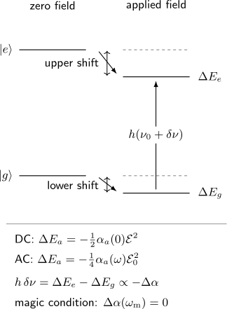
An applied field shifts both levels. A transition responds to the difference $\Delta\alpha=\alpha_e-\alpha_g$, not to either level polarizability alone. For a monochromatic field, the coefficient depends on frequency; at a magic frequency $\Delta\alpha(\omega_{\mathrm m})=0$ to leading electric-dipole order.

Differential Shifts, Traps, and Magic Conditions

Here the cancellation conditions are used to interpret atomic spectra and traps. Their multilevel computation, polarization dependence, root uncertainty, and loss diagnostics are developed on Dynamic Polarizability.

Let $|g\rangle$ and $|e\rangle$ define a transition of unperturbed frequency $\nu_0$. In a static scalar field,

$$\begin{aligned} h\,\delta\nu^{\mathrm{dc}} &=\Delta E_e-\Delta E_g\\ &=-\frac12 \Delta\alpha(0)\mathcal E^2, \end{aligned}$$

where

$$\Delta\alpha=\alpha_e-\alpha_g.$$

The line can move upward even when both levels move downward: only their difference determines the observed frequency.

For a monochromatic plane wave in vacuum, the cycle-averaged intensity associated with peak electric field $\mathcal E_0$ is

$$I = \frac12c\epsilon_0\mathcal E_0^2.$$

The scalar optical potential is therefore

$$U_n(\mathbf r) = -\frac{ \alpha_n(\omega) }{ 2c\epsilon_0 } I(\mathbf r),$$

and the dipole force is $\mathbf F=-\boldsymbol\nabla U_n$. Where $\alpha_n(\omega)>0$, atoms seek high intensity; where $\alpha_n(\omega)<0$, they seek low intensity. The common “red-detuned attracts, blue-detuned repels” rule is a useful two-level mnemonic, but the sign of the full multilevel polarizability is the actual criterion.

The differential light shift is

$$\delta\nu^{\mathrm{ac}} = -\frac{ \Delta\alpha(\omega) }{ 2hc\epsilon_0 }I.$$

A magic frequency $\omega_{\mathrm m}$ for a chosen pair of states and experimental geometry satisfies

$$\Delta\alpha(\omega_{\mathrm m})=0.$$

To leading order, the trap then confines both states while leaving their transition frequency insensitive to intensity. Magic wavelengths enabled optical lattice clocks by separating mechanical confinement from the dominant differential electric-dipole light shift.

A tune-out frequency for one state instead satisfies

$$\alpha_n(\omega_{\mathrm{to}})=0.$$

It cancels that state’s leading scalar optical potential. A tune-out condition is not generally magic for a transition, and a magic condition does not imply that either state has zero shift.

Neither condition removes every systematic effect. Vector and tensor shifts, imperfect polarization, hyperpolarizability, magnetic-dipole and electric-quadrupole couplings, photon scattering, motion through an inhomogeneous field, and higher-order intensity dependence can remain. “Magic” always names a specified cancellation under stated conditions.

Spectroscopic and Experimental Interpretation

An observed Stark-shifted spectrum is generated by field-dressed eigenvalues and field-dressed transition amplitudes. Mixing can transfer oscillator strength to a nominally forbidden line, change polarization dependence, and create avoided crossings. A reliable forward model therefore proceeds in four stages:

1. Construct the internal Hamiltonian at the required resolution, including fine, hyperfine, Zeeman, and Stark terms that compete on the experimental scale.
2. Diagonalize in symmetry blocks and track both eigenvalues and eigenvectors as the field changes.
3. Compute transition matrix elements between the dressed states for the actual probe polarization and geometry.
4. Average over spatial field distributions, populations, motion, linewidths, and instrumental response before comparing with data.

For a transition with a leading scalar DC response in an unknown stray field, applying a calibrated bias gives

$$\nu(\boldsymbol{\mathcal E}_{\mathrm a}) = \nu_0 -\frac{\Delta\alpha}{2h} \left| \boldsymbol{\mathcal E}_{\mathrm a} +\boldsymbol{\mathcal E}_{\mathrm s} \right|^2.$$

Scanning one signed component produces a parabola whose vertex reveals the opposite component of the stray field. Repeating along independent axes reconstructs the vector field. Reversing the bias is especially useful: the part of the frequency difference odd in the applied field isolates the cross term with the stray field.

Optical-trap spectroscopy has an analogous intensity problem. Atoms sample different $I(\mathbf r)$, so a differential polarizability causes an inhomogeneous distribution of transition shifts and can broaden or asymmetrically distort a line. Measuring at several trap intensities, controlling polarization, and extrapolating to zero intensity separates a leading light shift from the unperturbed frequency. Operating near a magic condition reduces the slope but does not remove the need for an uncertainty budget.

Thermal electromagnetic radiation also produces AC Stark shifts over a broadband spectrum. At modest accuracy one may approximate the response by its static polarizability, but precision clocks require dynamic corrections and a measured radiation environment. A blackbody shift is not an unrelated effect; it is a thermally averaged dynamic Stark shift.

Finally, strong static fields can broaden levels by field ionization, and near-resonant optical fields produce scattering and power broadening. A fitted line center is trustworthy only when the line-shape model includes the relevant dissipative physics.

Common Mistakes

Inferring quadratic behavior from “an atom has parity”

Parity forbids a permanent dipole only for an isolated parity eigenstate. An exact or near opposite-parity degeneracy must be treated as a coupled model space and can show a linear regime.

Calling every linear shift a permanent dipole

In hydrogen, the field creates oriented superpositions inside a degenerate manifold. The individual field-dressed branches carry dipoles, while the zero-field parity basis does not.

Using a level polarizability for a spectral line

A transition shift uses $\Delta\alpha=\alpha_e-\alpha_g$. The common shift of both levels is invisible to the transition frequency.

Dropping continuum and core contributions without an error estimate

The polarizability sum is complete. Dominant-line approximations can be excellent, but their omitted tail and core terms must be bounded for precision work.

Mixing peak and RMS optical fields

With a peak field, the AC shift is $-\alpha\mathcal E_0^2/4$. With an RMS field, it is $-\alpha\mathcal E_{\mathrm{rms}}^2/2$.

Treating scalar, vector, and tensor coefficients as interchangeable

State labels and polarization geometry decide which irreducible components contribute. A scalar table entry cannot predict every magnetic-sublevel shift.

Using a dispersive shift arbitrarily close to resonance

Near resonance, population transfer, linewidths, and photon scattering accompany the level shift. A purely real conservative potential is then incomplete.

Assuming magic means shift-free

A magic condition cancels a specified differential coefficient, usually the leading scalar electric-dipole term. Higher multipoles, hyperpolarizability, polarization errors, and other systematics can survive.

Exercises

Exercise 1: Linear Stark splitting in hydrogen

Diagonalize the spinless hydrogen $n=2$ block

$$PVP = \begin{pmatrix} 0 & -3ea_0\mathcal E\\ -3ea_0\mathcal E & 0 \end{pmatrix}.$$

Find the eigenvalues, normalized eigenstates, and induced dipoles $-\partial E/\partial\mathcal E$.

Solution

The symmetric and antisymmetric combinations diagonalize the matrix. One convenient labeling is

$$\begin{aligned} |+\rangle &= \frac{|2s\rangle-|2p,0\rangle}{\sqrt2}, \\ |-\rangle &= \frac{|2s\rangle+|2p,0\rangle}{\sqrt2}. \end{aligned}$$

They have shifts

$$\Delta E_+=+3ea_0\mathcal E, \qquad \Delta E_-=-3ea_0\mathcal E.$$

Therefore

$$\langle d_z\rangle_+ = -\frac{\partial E_+}{\partial\mathcal E} =-3ea_0,$$

and $\langle d_z\rangle_-=+3ea_0$. Rephasing $|2p,0\rangle$ interchanges which superposition receives which label, but the two shifts and opposite dipoles are invariant as a set.

Exercise 2: A rubidium DC shift

Use $\alpha_0/h=0.0794\ \mathrm{Hz}/(\mathrm{V/cm})^2$ for the $^{87}\mathrm{Rb}$ $5^2S_{1/2}$ ground state. Find its shift at $30\ \mathrm{V/cm}$. If a transition has $\Delta\alpha/h=0.1223\ \mathrm{Hz}/(\mathrm{V/cm})^2$, find the transition-frequency shift at the same field.

Solution

For the ground level,

$$\begin{aligned} \Delta\nu_g &= -\frac12(0.0794)(30)^2\ \mathrm{Hz} \\ &=-35.73\ \mathrm{Hz}. \end{aligned}$$

The line shift uses the differential coefficient:

$$\begin{aligned} \delta\nu &= -\frac12(0.1223)(30)^2\ \mathrm{Hz} \\ &=-55.04\ \mathrm{Hz}. \end{aligned}$$

The second result is not obtained by using the ground-state shift alone; it already represents the upper-minus-lower response.

Exercise 3: Peak versus RMS amplitude

A far-detuned monochromatic field has peak amplitude $\mathcal E_0=200\ \mathrm{V/m}$ and produces a scalar AC shift $-\alpha(\omega)\mathcal E_0^2/4$. Express the same formula using the RMS field and show that the numerical shift is unchanged.

Solution

The RMS amplitude is

$$\mathcal E_{\mathrm{rms}} = \frac{200}{\sqrt2}\ \mathrm{V/m}.$$

Hence

$$\begin{aligned} -\frac12\alpha\mathcal E_{\mathrm{rms}}^2 &= -\frac12\alpha\frac{(200)^2}{2} \\ &= -\frac14\alpha(200)^2. \end{aligned}$$

The two expressions agree. Substituting $\mathcal E_{\mathrm{rms}}$ into the peak-amplitude formula would incorrectly reduce the shift by another factor of two.

Exercise 4: Magic and tune-out frequencies

At a frequency $\omega_1$, suppose $\alpha_g=120$ and $\alpha_e=120$ in the same units. At another frequency $\omega_2$, suppose $\alpha_g=0$ and $\alpha_e=-40$. Which frequency is magic for the $g\leftrightarrow e$ transition, and which is a tune-out frequency for $|g\rangle$? What optical potential remains for each state?

Solution

At $\omega_1$,

$$\Delta\alpha=\alpha_e-\alpha_g=0,$$

so the frequency is magic for the transition. Both states still experience the same nonzero optical potential proportional to $-120I$; the trap remains while the leading differential shift cancels.

At $\omega_2$, $\alpha_g=0$, so this is a tune-out frequency for the ground state. The excited state still has a nonzero potential proportional to $+40I$ because its polarizability is negative. Since $\Delta\alpha=-40$, the transition is not magic.

Exercise 5: Measuring a stray electric field

A one-dimensional bias field $\mathcal E_{\mathrm a}$ is applied along an unknown stray component $\mathcal E_{\mathrm s}$. Show where the quadratic Stark curve

$$\begin{aligned} \nu(\mathcal E_{\mathrm a}) &= \nu_0-C\mathcal E_{\mathrm{tot}}^2, \\ \mathcal E_{\mathrm{tot}} &= \mathcal E_{\mathrm a}+\mathcal E_{\mathrm s}. \end{aligned}$$

has its vertex. Also evaluate $\nu(+E)-\nu(-E)$.

Solution

Differentiate with respect to the applied field:

$$\frac{d\nu}{d\mathcal E_{\mathrm a}} = -2C\mathcal E_{\mathrm{tot}}.$$

The vertex occurs at

$$\mathcal E_{\mathrm a}=-\mathcal E_{\mathrm s}.$$

For equal and opposite biases,

$$\begin{aligned} \nu(+E)-\nu(-E) &=-C(E+\mathcal E_{\mathrm s})^2\\ &\quad+C(-E+\mathcal E_{\mathrm s})^2\\ &=-4CE\mathcal E_{\mathrm s}. \end{aligned}$$

The reversal difference isolates the cross term and is linear in the stray component. Biases along several independent directions are required to reconstruct a three-dimensional stray field.

Cross-Links

• Common Atomic Hamiltonians distinguishes explicit dipole coupling from an eliminated-state polarizability term and routes other atomic operators.
• Atomic Physics
• Hydrogen as the Atomic Prototype
• Alkali Atoms
• Rydberg Atoms Basics
• Fine Structure
• Hyperfine Structure
• Zeeman Effect in Atoms
• Stark Effect as a Perturbation Example
• Stark Shift in a Two-Level Approximation
• Dynamic Polarizability
• Dipole Transitions
• Selection Rules
• Scalar, Vector, and Tensor Operators
• Stark Effect glossary entry
• Spectroscopy
• AMO Physics Roadmap

References

1. J. Stark, “Observation of the Separation of Spectral Lines by an Electric Field,” Nature 92, 401 (1913), DOI: 10.1038/092401b0.
2. J. Stark, “Beobachtungen über den Effekt des elektrischen Feldes auf Spektrallinien. I. Quereffekt,” Annalen der Physik 348, 965–982 (1914), DOI: 10.1002/andp.19143480702.
3. E. Schrödinger, “Quantisierung als Eigenwertproblem. Dritte Mitteilung: Störungstheorie, mit Anwendung auf den Starkeffekt der Balmerlinien,” Annalen der Physik 385, 437–490 (1926), DOI: 10.1002/andp.19263851302.
4. A. Dalgarno and J. T. Lewis, “The Exact Calculation of Long-Range Forces between Atoms by Perturbation Theory,” Proceedings of the Royal Society A 233, 70–74 (1955), DOI: 10.1098/rspa.1955.0246.
5. J. Mitroy, M. S. Safronova, and C. W. Clark, “Theory and applications of atomic and ionic polarizabilities,” Journal of Physics B 43, 202001 (2010), DOI: 10.1088/0953-4075/43/20/202001; arXiv:1004.3567.
6. R. Grimm, M. Weidemüller, and Y. B. Ovchinnikov, “Optical Dipole Traps for Neutral Atoms,” Advances in Atomic, Molecular, and Optical Physics 42, 95–170 (2000), DOI: 10.1016/S1049-250X(08)60186-X; arXiv:physics/9902072.
7. F. Le Kien, P. Schneeweiss, and A. Rauschenbeutel, “Dynamical polarizability of atoms in arbitrary light fields: general theory and application to cesium,” European Physical Journal D 67, 92 (2013), DOI: 10.1140/epjd/e2013-30729-x; arXiv:1211.2673.
8. M. S. Safronova, B. Arora, and C. W. Clark, “Frequency-dependent polarizabilities of alkali-metal atoms from ultraviolet through infrared spectral regions,” Physical Review A 73, 022505 (2006), DOI: 10.1103/PhysRevA.73.022505; arXiv:physics/0508087.
9. H. Katori, M. Takamoto, V. G. Pal’chikov, and V. D. Ovsiannikov, “Ultrastable Optical Clock with Neutral Atoms in an Engineered Light Shift Trap,” Physical Review Letters 91, 173005 (2003), DOI: 10.1103/PhysRevLett.91.173005.
10. M. Takamoto and H. Katori, “Spectroscopy of the $^1S_0$–$^3P_0$ Clock Transition of $^{87}\mathrm{Sr}$ in an Optical Lattice,” Physical Review Letters 91, 223001 (2003), DOI: 10.1103/PhysRevLett.91.223001.
11. D. A. Steck, $^{87}$Rb D Line Data, revision 2.3.4, 8 August 2025, accessed 2026-07-21.
12. C. J. Foot, Atomic Physics, Oxford University Press, 2005.
13. H. Friedrich, Theoretical Atomic Physics, 4th ed., Springer, 2017.
14. C. Cohen-Tannoudji, J. Dupont-Roc, and G. Grynberg, Atom–Photon Interactions: Basic Processes and Applications, Wiley, 1992.