Common Atomic Hamiltonians

An atomic Hamiltonian is more than a recognizable string of kinetic, Coulomb, and angular-momentum terms. It is a contract specifying the degrees of freedom, unit system, approximation order, external controls, reference frame, and operators retained in the model. Two papers can print nearly the same equation while predicting different quantities because one clamps the nucleus, one includes recoil, one works in a rotating frame, or one has already projected into a fine- or hyperfine-resolved manifold.

This page is the comparison and diagnostic index for common atomic Hamiltonians. It supplies compact forms, term meanings, regime tests, surviving symmetries, and routing links. The specialist pages linked from each section own derivations, spectra, experiments, and detailed error analysis.

Canonical Scope

Use this entry to answer:

1. What physical degrees of freedom does the displayed Hamiltonian retain?
2. Is it written in SI, Hartree atomic units, frequency units, or a rotating frame?
3. Which terms are fundamental at the chosen level and which are effective after projection or elimination?
4. Which quantum numbers remain exact?
5. What energy ratio decides whether a term is perturbative?
6. Could two terms count the same physics twice?

The AMO Model Index starts from a wider choice of degrees of freedom, including open-system and field models. This page begins after an atomic description has been chosen and identifies its operator content.

It does not reproduce the exact hydrogen solution, derive central-field or Hartree–Fock equations, calculate fine or hyperfine constants, or develop field-dressed and Rydberg dynamics in full. Those topics retain one canonical home each.

Hamiltonian Declaration

Before using a compact equation, record the following ledger.

Item	Question that must be answered
system	isotope, nuclear charge, ionization stage, number of electrons
Hilbert space	electronic coordinates only, nuclear spin, center-of-mass motion, photon modes, or selected levels
statistics	antisymmetric electronic subspace and any nuclear exchange symmetry
coordinates	laboratory, center-of-mass, relative, body-fixed, or lattice-site coordinates
units	SI, Hartree, Rydberg, hertz, or angular-frequency units
baseline	Schrödinger–Coulomb, Dirac–Coulomb, fitted model potential, or another reference
corrections	recoil, Breit, radiative, finite-size, hyperfine, and external-field terms retained
field convention	direction, amplitude, polarization, gauge, and static or time-dependent character
frame	laboratory, interaction, or rotating frame; detuning sign
model space	complete coordinate problem or projected manifold
energy zero	ionization threshold, term centroid, rotating-frame zero, or code-specific offset
approximation order	perturbative order and discarded terms

A useful notation is

$$H_{\mathrm{declared}} = H_{\mathrm{base}} +\sum_a \delta H_a,$$

but this sum is meaningful only when the terms were derived in one consistent partition. For example, a fitted effective potential may already contain scalar relativistic or core-polarization effects. Adding the same correction again is double counting.

Master Atomic Decomposition

For orientation, an atomic Hamiltonian may be organized schematically as

$$\begin{aligned} H_{\mathrm{atom}} ={}&H_{\mathrm C} +H_{\mathrm{recoil}} +H_{\mathrm{rel}}\\ &+H_{\mathrm{hfs}} +H_{\mathrm{ext}} +\delta H_{\mathrm{rad}} +\cdots . \end{aligned}$$

The pieces have different physical roles:

Layer	Typical content	Canonical destination
$H_{\mathrm C}$	nonrelativistic kinetic energy and Coulomb interactions	hydrogen and multi-electron pages
$H_{\mathrm{recoil}}$	reduced mass, mass polarization, higher recoil	isotope and precision treatments
$H_{\mathrm{rel}}$	mass–velocity, Darwin, spin–orbit, Breit, or a Dirac baseline	Fine Structure
$H_{\mathrm{hfs}}$	magnetic-dipole, electric-quadrupole, higher nuclear multipoles	Hyperfine Structure
$H_{\mathrm{ext}}$	electric, magnetic, optical, and gradient couplings	Stark, Zeeman, and light–matter pages
$\delta H_{\mathrm{rad}}$	self-energy, vacuum polarization, radiative recoil	Lamb Shift Overview

This is a bookkeeping hierarchy, not a claim that every term is separately observable. Effective-Hamiltonian conventions can move contributions between rows while leaving the final spectrum unchanged to the stated order.

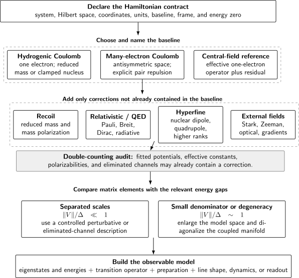
An atomic model is assembled in layers. The ratio $\lVert V\rVert/\Delta$ decides whether a correction may be eliminated perturbatively or whether its coupled manifold belongs in the retained Hamiltonian. Effective terms require a double-counting audit before the observable model is constructed.

Hydrogenic Hamiltonian

Relative-coordinate form

For one electron and a point nucleus of charge $+Ze$, separation of the center-of-mass motion gives the nonrelativistic relative Hamiltonian

$$H_{\mathrm C} =\frac{\mathbf p^2}{2\mu} -\frac{Ze^2}{4\pi\varepsilon_0r},$$

where

$$\mu =\frac{m_eM}{m_e+M}$$

is the electron–nucleus reduced mass. This model retains Coulomb binding and leading kinematic recoil through $\mu$. It omits relativity, nuclear size, radiative shifts, hyperfine structure, and external fields.

In standard Hartree atomic units,

$$H_{\mathrm C} =-\frac{m_e}{2\mu}\nabla^2-\frac{Z}{r}.$$

For a clamped or infinitely heavy nucleus, $\mu\to m_e$ and

$$H_{\infty} =-\frac12\nabla^2-\frac{Z}{r}.$$

The bound energies of this declared model are

$$E_n =-\frac{\mu}{m_e} \frac{Z^2}{2n^2}E_{\mathrm h}.$$

The Hydrogen Atom page owns the exact bound-state solution. Hydrogen as Atomic Prototype owns the correction ladder needed to compare the ideal model with a measured hydrogen line.

Diagnostic labels

For the spin-independent Coulomb Hamiltonian, $n,\ell,m$ label spatial eigenstates and spin is a spectator. The pure $1/r$ potential has an additional dynamical symmetry, so the nonrelativistic bound energy depends only on $n$. A generic central potential keeps rotational symmetry but loses this accidental $\ell$ degeneracy.

The phrase “hydrogenic Hamiltonian” should state at least:

• point or extended nucleus;
• infinite or finite nuclear mass;
• one electron or an effective one-active-electron model;
• nonrelativistic Schrödinger or relativistic Dirac baseline; and
• whether the printed energy is a total energy, binding magnitude, or transition energy.

Multi-Electron Coulomb Hamiltonian

For $N$ nonrelativistic electrons and a clamped point nucleus at the origin, the SI Hamiltonian is

$$\begin{aligned} H_{\mathrm C} ={}& \sum_{i=1}^{N} \left[ \frac{\mathbf p_i^2}{2m_e} -\frac{Ze^2}{4\pi\varepsilon_0r_i} \right]\\ &+ \sum_{i<j} \frac{e^2}{4\pi\varepsilon_0r_{ij}}. \end{aligned}$$

In Hartree atomic units this becomes

$$\begin{aligned} H_{\mathrm C} ={}& \sum_{i=1}^{N} \left( -\frac12\nabla_i^2-\frac{Z}{r_i} \right)\\ &+\sum_{i<j}\frac1{r_{ij}}. \end{aligned}$$

The physical electronic state belongs to the antisymmetric subspace:

$$P_{ij}\Psi=-\Psi.$$

The electron–electron term couples coordinates, so the exact eigenstate is not generally a single product of one-electron orbitals. The canonical Multi-Electron Atoms chapter develops antisymmetry, shell structure, mean fields, exchange, correlation, and coupling schemes.

Finite nuclear mass

After separating the overall center of mass, a convenient recoil operator contains

$$H_{\mathrm{recoil}}^{(1)} =\frac1{2M} \left( \sum_i\mathbf p_i \right)^2.$$

Expanding the square produces one-electron normal-mass terms and the two-electron mass-polarization term:

$$\begin{aligned} H_{\mathrm{recoil}}^{(1)} ={}& \sum_i\frac{\mathbf p_i^2}{2M}\\ &+\frac1M \sum_{i<j} \mathbf p_i\cdot\mathbf p_j. \end{aligned}$$

This expression assumes momenta conjugate to electron coordinates relative to the nucleus. Coordinate and sign conventions must be checked before transplanting it into another representation. Precision isotope shifts also contain relativistic recoil, field shifts, and nuclear-polarization effects.

What the compact form omits

The Schrödinger–Coulomb Hamiltonian omits:

• spin-dependent interactions;
• finite nuclear charge and magnetization distributions;
• transverse-photon and retardation effects;
• radiative QED corrections;
• external fields and collisions; and
• the numerical representation, basis, and truncation.

A calculation can solve the displayed Hamiltonian poorly, or solve a more complete Hamiltonian accurately. Always separate model error from numerical error.

Central-Field Reference Hamiltonian

The central-field approximation chooses a separable reference

$$H_0 =\sum_i h_{\mathrm{cf}}(i),$$

with

$$h_{\mathrm{cf}} =-\frac12\nabla^2+V_{\mathrm{cf}}(r)$$

in Hartree units. The exact identity

$$H_{\mathrm C}=H_0+H_{\mathrm{res}}$$

then defines

$$\begin{aligned} H_{\mathrm{res}} ={}& \sum_{i<j}\frac1{r_{ij}}\\ &+\sum_i \left[ -\frac{Z}{r_i} -V_{\mathrm{cf}}(r_i) \right]. \end{aligned}$$

If

$$V_{\mathrm{cf}}(r) =-\frac{Z}{r}+U(r),$$

the residual simplifies to

$$H_{\mathrm{res}} =\sum_{i<j}\frac1{r_{ij}} -\sum_iU(r_i).$$

The subtraction is essential: once an average interaction $U$ has been added to $H_0$, it must be removed from the residual before the full electron–electron interaction is restored.

Meaning of the reference

A local central field guarantees

$$[h_{\mathrm{cf}},L^2]=0, \qquad [h_{\mathrm{cf}},L_z]=0,$$

and orbitals can be labeled by $n,\ell,m$. It does not guarantee hydrogenic degeneracy between different $\ell$, nor does it make orbital energies equal to exact ionization or excitation energies.

The origin of $V_{\mathrm{cf}}$ must be stated:

Construction	What it represents
fitted model potential	selected empirical or high-level observables
Hartree field	local direct electrostatic mean field
Hartree–Fock operator	direct field plus generally nonlocal exchange
density-functional potential	chosen exchange-correlation functional
frozen-core potential	valence motion after a declared core reduction

These operators can generate similar orbital labels while carrying different many-body content. Central-Field Approximation owns the screening, self-consistency, quantum-defect, and validation diagnostics.

Fine-Structure Operators

One-electron Pauli correction

For a spin-$1/2$ electron in a static central potential energy $V(r)$, the nonrelativistic reference is

$$H_0 =\frac{\mathbf p^2}{2m_e}+V(r).$$

Through order $1/c^2$, the leading one-electron correction is

$$H_{\mathrm{fs}}^{(1)} =H_{\mathrm{mv}}+H_{\mathrm{so}}+H_D,$$

with

$$H_{\mathrm{mv}} =-\frac{\mathbf p^4}{8m_e^3c^2},$$ $$H_{\mathrm{so}} =\frac1{2m_e^2c^2} \frac1r\frac{dV}{dr} \mathbf L\cdot\mathbf S,$$

and

$$H_D =\frac{\hbar^2}{8m_e^2c^2} \nabla^2V.$$

$H_{\mathrm{mv}}$ is the relativistic kinetic correction, $H_{\mathrm{so}}$ is the spin–orbit term including the Thomas factor, and $H_D$ is the Darwin term. Spin–orbit coupling is therefore one part of fine structure, not a synonym for the entire correction.

In Hartree atomic units, $c=\alpha^{-1}$ and the same terms become

$$\begin{aligned} H_{\mathrm{mv}} &=-\frac{\alpha^2}{8}\mathbf p^4,\\ H_{\mathrm{so}} &=\frac{\alpha^2}{2r} \frac{dV}{dr} \mathbf L\cdot\mathbf S,\\ H_D &=\frac{\alpha^2}{8}\nabla^2V. \end{aligned}$$

Here angular momenta and momenta are represented in their Hartree-unit numerical form with $\hbar=1$.

Point-Coulomb spin–orbit term

For

$$V(r) =-\frac{Ze^2}{4\pi\varepsilon_0r},$$

the SI spin–orbit operator is

$$H_{\mathrm{so}} = \frac{Ze^2} {8\pi\varepsilon_0m_e^2c^2r^3} \mathbf L\cdot\mathbf S.$$

The angular identity

$$2\mathbf L\cdot\mathbf S =J^2-L^2-S^2$$

diagonalizes this operator in a fixed $\ell,s,j$ manifold. A rotationally invariant spin–orbit interaction preserves $J,m_J$ and parity, while $L$ and $S$ can cease to be exact in general many-electron intermediate coupling.

Multi-electron boundary

Many-electron fine structure can also contain spin–other-orbit, mutual spin–orbit, spin–spin, and orbit–orbit terms, or be described from a Dirac–Coulomb–Breit baseline. The one-electron Pauli form is controlled when momenta are nonrelativistic and $Z\alpha\ll1$. Heavy highly charged ions require a relativistic starting point rather than an uncontrolled sequence of low-order patches.

Fine Structure owns the derivation, hydrogenic spectrum, many-electron coupling, and boundaries of the expansion.

Zeeman Hamiltonians

Linear magnetic coupling

For a static field $\mathbf B$, a common leading energy Hamiltonian is

$$H_Z =\frac{\mu_{\mathrm B}}{\hbar} \left( g_L\mathbf L +g_S\mathbf S +g_I'\mathbf I \right) \cdot\mathbf B.$$

The electronic coefficients $g_L$ and $g_S$ are positive in this energy convention; the negative electron charge is already included in $-\boldsymbol\mu\cdot\mathbf B$. The nuclear coefficient

$$g_I' =-g_I\frac{\mu_{\mathrm N}}{\mu_{\mathrm B}}$$

is defined on the Bohr-magneton scale. Confusing it with the nuclear $g$ factor paired with $\mu_{\mathrm N}$ introduces a factor near $m_p/m_e$ and can reverse a sign.

If $\mathbf B=B\hat{\mathbf z}$ and fine structure is dominant over the magnetic interaction, projection into an isolated $J$ level gives

$$\Delta E =g_J\mu_{\mathrm B}m_JB.$$

If hyperfine coupling is also dominant over the magnetic interaction, projection into an isolated $F$ manifold gives

$$\Delta E =g_F\mu_{\mathrm B}m_FB.$$

These are first-order effective formulas, not replacements for the operator when the field mixes $J$ or $F$ manifolds.

Diamagnetic term

For a uniform field in the symmetric gauge,

$$\mathbf A =\frac12\mathbf B\times\mathbf r,$$

minimal coupling produces the one-electron diamagnetic term

$$H_{\mathrm{dia}} =\frac{e^2}{8m_e} \lvert\mathbf B\times\mathbf r\rvert^2.$$

It is quadratic in $B$. Second-order level shifts also arise from virtual mixing by the linear Zeeman operator. These are distinct contributions and must be combined consistently.

Field-regime test

The word “weak” is relative to a particular zero-field splitting:

Comparison	Useful labels	Treatment
$\mu_{\mathrm B}B\ll\Delta E_{\mathrm{hfs}}$	$F,m_F$	projected $g_F$ formula
$\mu_{\mathrm B}B\sim\Delta E_{\mathrm{hfs}}$	$m_F$ exact, $F$ mixed	diagonalize fixed-$m_F$ blocks
$\Delta E_{\mathrm{hfs}}\ll\mu_{\mathrm B}B\ll\Delta E_{\mathrm{fs}}$	$m_I,m_J$	hyperfine Paschen–Back basis
$\mu_{\mathrm B}B\sim\Delta E_{\mathrm{fs}}$	total axial projection	include neighboring $J$ levels

Zeeman Effect in Atoms owns Landé factors, Breit–Rabi crossover spectra, Paschen–Back regimes, polarization-resolved transitions, and experimental interpretation.

Stark Hamiltonians

Uniform electric field

In the long-wavelength electric-dipole approximation,

$$H_E(t) =-\mathbf d\cdot\boldsymbol{\mathcal E}(t),$$

where the total dipole operator is

$$\mathbf d=\sum_a q_a\mathbf r_a$$

relative to a declared origin. For one electron relative to a fixed nucleus,

$$\mathbf d=-e\mathbf r.$$

For a neutral atom the total internal dipole is independent of an overall origin shift. For an ion it is not: separate center-of-mass and internal coordinates before interpreting a uniform-field coupling, and state which motion the model retains.

For a static field $\boldsymbol{\mathcal E}=\mathcal E\hat{\mathbf z}$,

$$H_E=-\mathcal E d_z.$$

The dipole approximation requires the field to vary little over the atomic size. Field gradients introduce quadrupole and higher-multipole couplings.

Perturbative scale

For a state $|a\rangle$ coupled to $|b\rangle$, define

$$\eta_{ab} = \frac{ \mathcal E \lvert\langle a|d_z|b\rangle\rvert }{ \lvert E_a^{(0)}-E_b^{(0)}\rvert }.$$

If $\eta_{ab}\ll1$ for all states outside the retained manifold, perturbation theory is controlled. If a denominator is small, include those states in the model space and diagonalize.

For an isolated nondegenerate parity eigenstate, the leading static shift is usually

$$\Delta E_a =-\frac12\alpha_a(0)\mathcal E^2.$$

This is a derived effective energy after virtual opposite-parity states have been eliminated. It is not an additional microscopic interaction to add on top of an explicit dipole-coupled basis, or the same mixing is counted twice.

At exact opposite-parity degeneracy, the projected two-state Hamiltonian

$$H_{\mathrm{eff}} = \begin{pmatrix} -\delta/2 & -d\mathcal E\\ -d\mathcal E & \delta/2 \end{pmatrix}$$

has a linear splitting when $\delta=0$. Thus parity symmetry does not forbid the linear Stark effect inside a degenerate manifold.

Stark Effect in Atoms owns static and dynamic polarizability, hydrogenic degeneracy, scalar/vector/tensor responses, magic conditions, and experimental field calibration.

Hyperfine Hamiltonians

Hyperfine structure couples nuclear electromagnetic multipoles to electronic fields at the nucleus. A rotationally invariant expansion is

$$H_{\mathrm{hfs}} =\sum_{k\ge1} T_{\mathrm{nuc}}^{(k)} \cdot T_{\mathrm{el}}^{(k)}.$$

The leading $k=1$ term is magnetic dipole; $k=2$ is electric quadrupole.

Magnetic-dipole term

Within an isolated electronic level of angular momentum $J$,

$$H_{\mathrm{M1}} =\frac{A}{\hbar^2} \mathbf I\cdot\mathbf J.$$

With

$$\mathbf F=\mathbf I+\mathbf J$$

and

$$K =F(F+1)-I(I+1)-J(J+1),$$

the first-order energy is

$$E_F^{\mathrm{M1}} =\frac A2K.$$

$A$ includes both the nuclear magnetic moment and the electronic magnetic field at the nucleus. It can be positive or negative and is state- and isotope-specific.

Electric-quadrupole term

For $I\ge1$ and $J\ge1$, the conventional first-order quadrupole energy is

$$\begin{aligned} E_F^{\mathrm{E2}} &=B\frac{N_{IJF}}{D_{IJ}},\\ N_{IJF} &=\frac34K(K+1) -I(I+1)J(J+1),\\ D_{IJ} &=2I(2I-1)J(2J-1). \end{aligned}$$

The standard dipole-plus-quadrupole model is

$$E_F^{\mathrm{hfs}} =\frac A2K+E_F^{\mathrm{E2}}.$$

For $I<1$ or $J<1$, the first-order $B$ term is absent. Databases often quote $A/h$ and $B/h$ in MHz while labeling the columns simply $A$ and $B$. Determine whether the constants are energies or frequencies before using them.

Hyperfine plus magnetic field

When the Zeeman energy is not small compared with hyperfine intervals, use

$$H =H_{\mathrm{hfs}}+H_Z$$

and diagonalize in a basis such as $|I,m_I\rangle|\gamma,J,m_J\rangle$ at fixed axial projection. Substituting a field-dependent $g_F$ into a weak-field formula is not equivalent.

Hyperfine Structure owns the microscopic interactions, interval rules, hydrogen and alkali examples, clock transitions, and field crossovers.

Rydberg Interaction Models

Rydberg interactions are effective atomic Hamiltonians obtained after choosing asymptotic pair states, multipole order, geometry, and external fields.

Dipole–dipole operator

At separation $R$ much larger than the electronic-cloud size, the leading electric dipole–dipole operator is

$$\begin{aligned} V_{dd}(\mathbf R) ={}& \frac1{4\pi\varepsilon_0R^3} \left[ \mathbf d_1\cdot\mathbf d_2\right.\\ &\left. -3(\mathbf d_1\cdot\hat{\mathbf R}) (\mathbf d_2\cdot\hat{\mathbf R}) \right]. \end{aligned}$$

It is an anisotropic operator in the magnetic-sublevel pair space, not a universal scalar potential.

Two-channel pair Hamiltonian

If a prepared pair state $|rr\rangle$ couples mainly to $|r'r''\rangle$, subtract the energy of $|rr\rangle$ and write

$$H_{\mathrm{pair}} = \begin{pmatrix} 0 & V_{dd}\\ V_{dd}^* & \Delta_F \end{pmatrix},$$

where

$$\Delta_F =E_{r'}+E_{r''}-2E_r$$

is the Förster defect.

For

$$\lvert V_{dd}\rvert\ll\lvert\Delta_F\rvert,$$

the shift of the prepared channel is

$$\Delta E_{rr} \simeq-\frac{\lvert V_{dd}\rvert^2}{\Delta_F} =\frac{C_6}{R^6}.$$

The sign of $C_6$ follows from the channel defects and matrix elements. Near resonance,

$$\lvert\Delta_F\rvert \lesssim \lvert V_{dd}\rvert,$$

the channels must be diagonalized and the leading splitting scales as $C_3/R^3$.

Driven two-level array

After selecting one ground state $|g_i\rangle$ and one Rydberg state $|r_i\rangle$, transforming to a rotating frame, and adopting the rotating- wave approximation, a common coherent array model is

$$\begin{aligned} \frac H\hbar ={}& \sum_i \frac{\Omega_i}{2} \left( e^{i\phi_i}|r_i\rangle\langle g_i| +\mathrm{h.c.} \right)\\ &-\sum_i\Delta_i n_i +\sum_{i<j} \frac{V_{ij}}{\hbar}n_in_j, \end{aligned}$$

with

$$n_i=|r_i\rangle\langle r_i|.$$

The sign shown uses

$$\Delta_i=\omega_{L,i}-\omega_{rg,i}.$$

Some sources define the opposite detuning. The drive amplitude may also be defined with or without the factor $1/2$.

This model omits leakage levels, intermediate-state scattering, motion, position-dependent phases, state-changing pair interactions, dissipation, and readout error unless those are added explicitly. Rydberg Atoms Basics owns the scaling and pair-channel physics; Rydberg Blockade owns finite-blockade dynamics and projected many-body limits.

Perturb or Diagonalize?

The important question is not whether a correction “looks small” in absolute units, but whether its matrix elements are small relative to the energy denominators connecting retained and omitted states.

Let $P$ project onto a chosen model space and $Q=1-P$. A schematic energy-dependent effective Hamiltonian is

$$\begin{aligned} H_{\mathrm{eff}}(E) ={}&PHP\\ &+PHQ \frac1{E-QHQ} QHP. \end{aligned}$$

Expanding the resolvent is controlled only away from small denominators. This one structure underlies:

• scalar Stark shifts after opposite-parity states are eliminated;
• van der Waals Rydberg shifts after off-resonant pair channels are eliminated;
• effective hyperfine or Zeeman operators within an isolated manifold; and
• central-field residual corrections within a truncated configuration space.

Use the following decision rule:

Ratio or situation	Action
$\lVert V\rVert/\Delta\ll1$ and no relevant degeneracy	perturbation theory may be controlled
$\lVert V\rVert/\Delta$ not small	enlarge the model space and diagonalize
exact or symmetry-protected degeneracy	diagonalize $PVP$ before expanding
omitted continuum near threshold	include continuum coupling or resonance methods
non-Hermitian loss or driving	use an open-system or effective non-Hermitian model with stated limits

An avoided crossing is often evidence that the original diagonal labels have become basis labels. Follow the eigenvectors continuously or use exact symmetry labels rather than assigning levels solely by zero-field names.

Symmetry and Good-Label Table

“Good quantum number” means that the declared Hamiltonian commutes with the corresponding observable and that the relevant eigenvalue distinguishes the states under discussion.

Declared model	Typically exact labels or sectors	Labels that may fail
one-electron Coulomb, no spin terms	$\ell,m$, parity; $n$ labels bound energy	fine-, hyperfine-, and field-dressed labels absent
spin-independent multi-electron Coulomb	$L,S$, their projections, parity; $J$ can also be formed	configurations and orbital occupations need not be exact
local central field	one-electron $\ell,m$ and parity	hydrogenic degeneracy across $\ell$
rotationally invariant fine structure	total $J,m_J$, parity	separate $L,S$ in intermediate coupling
zero-field hyperfine	$F,m_F$, parity	separate $m_I,m_J$
uniform dc electric field along $z$	axial projection $m$	parity and usually total angular-momentum magnitude
uniform dc magnetic field along $z$	axial total projection and parity	$F$ or $J$ across Paschen–Back crossovers
crossed nonparallel electric and magnetic fields	only surviving discrete symmetries, if any	a universal magnetic projection
axial Rydberg pair problem	total axial projection and exchange sectors when applicable	individual atomic $m$ under anisotropic mixing

Degeneracy alone does not imply a symmetry label, and a familiar label can remain useful approximately after it ceases to be exact. Report dominant components or expectation values when assigning mixed states.

Units, Gauges, and Frames

Energy versus frequency Hamiltonians

Some AMO literature writes $H$ in energy units; other literature writes $H/\hbar$ in angular-frequency units. These equations are not numerically identical:

$$i\hbar\frac{d}{dt}|\psi\rangle =H|\psi\rangle$$

becomes

$$i\frac{d}{dt}|\psi\rangle =\frac H\hbar|\psi\rangle.$$

A matrix entry labeled “MHz” may mean $H/h$ in cycles per second or $H/\hbar$ with a convention that quotes $\Omega/(2\pi)$. State the defining equation.

The Atomic Units reference gives the Hartree conversion and dimensional restoration rules.

Length and velocity gauges

For a time-dependent electromagnetic field, the dipole coupling

$$-\mathbf d\cdot\boldsymbol{\mathcal E}(t)$$

is a length-gauge form. A minimal-coupling or velocity-gauge Hamiltonian uses $\mathbf p-q\mathbf A$. The formulations are related by a unitary gauge transformation in a complete, consistently transformed theory. Truncated bases, omitted $A^2$ terms, or inconsistent observables can break numerical gauge agreement.

Do not add a length-gauge dipole term and a velocity-gauge $\mathbf p\cdot\mathbf A$ term for the same field unless a derivation explicitly requires both.

Rotating frames

A rotating-frame transformation changes the Hamiltonian by

$$H_{\mathrm{rot}} =UHU^\dagger +i\hbar\dot U U^\dagger.$$

The second term generates detunings and frame-dependent energy zeros. A rotating-wave approximation then discards selected fast terms. Report:

• the unitary $U(t)$ or enough information to reconstruct it;
• the sign definition of detuning;
• whether $\Omega$ is a matrix element or a Rabi angular frequency;
• which counter-rotating and light-shift terms were dropped; and
• the observable transformation back to the laboratory frame.

Assembly and Validation Workflow

1. Choose the baseline

State whether the zeroth-order model is Schrödinger–Coulomb, Dirac–Coulomb, a central-field operator, or a projected few-level Hamiltonian.

2. Inventory retained degrees of freedom

List electronic coordinates, nuclear spin, motion, field modes, and selected internal states. A term cannot act on a degree of freedom absent from the Hilbert space.

3. Order the energy scales

Construct a hierarchy such as

$$\Delta E_{\mathrm{gross}}, \quad \Delta E_{\mathrm{fs}}, \quad \Delta E_{\mathrm{hfs}}, \quad \mu_{\mathrm B}B, \quad d\mathcal E, \quad \hbar\Omega, \quad \hbar\Gamma.$$

The ordering determines useful labels and which manifolds must be diagonalized together.

4. Check units and signs

Verify charge signs, $h$ versus $\hbar$, Hartree versus Rydberg, peak versus root-mean-square field, detuning sign, and energy zero.

5. Audit double counting

Ask whether an effective constant, fitted potential, polarizability, pseudopotential, or eliminated channel already contains a correction being added explicitly.

6. Test structural limits

At minimum, verify:

• Hermiticity for a closed coherent model;
• dimensions of every term;
• the zero-field or zero-coupling limit;
• parity and projection blocks predicted by symmetry;
• trace or centroid identities where applicable;
• convergence under basis and model-space enlargement; and
• agreement with one independent benchmark.

7. Connect to an observable

Level eigenvalues are not automatically spectral line positions, and a line position is not a line strength. Add the initial and final states, transition operator, selection rules, line shape, preparation, and detection model needed for the measured quantity.

Common Mistakes

Writing an equation without its Hilbert space

$A\mathbf I\cdot\mathbf J$ is meaningless if nuclear spin was projected out, and $C_6/R^6$ is not an operator on unspecified pair states.

Treating every correction as independently additive

Effective potentials and fitted constants can already contain pieces of correlation, relativity, or core response.

Calling spin–orbit coupling the whole fine structure

Mass–velocity, Darwin, and many-electron relativistic terms can contribute at the same order.

Using weak-field Landé formulas through a crossover

When Zeeman and hyperfine or fine-structure scales are comparable, diagonalize the coupled Hamiltonian.

Adding a quadratic Stark shift to an explicit dipole basis

The polarizability shift is generated by virtual dipole coupling. Adding both without a subtraction double counts that response.

Using a scalar Rydberg interaction without a pair-state declaration

$C_6$ depends on state, magnetic sublevel, geometry, fields, and nearby channels.

Ignoring the energy zero

Total energies, binding energies, orbital eigenvalues, rotating-frame quasienergies, and transition frequencies are different objects.

Mixing energy and frequency constants

A hyperfine constant quoted in MHz may denote $A/h$, while a coherent-control Hamiltonian may use $A/\hbar$. The difference is $2\pi$.

Mixing gauges in a truncated calculation

Length- and velocity-gauge results agree only after states, operators, and truncations are transformed consistently.

Assuming a basis label remains exact

$F$, $J$, $L$, $S$, and configurations can become approximate labels under field or interaction mixing. Use exact symmetry sectors and report composition.

Exercises

Exercise 1: Reduced-mass hydrogenic Hamiltonian

Write the one-electron Coulomb Hamiltonian in standard Hartree atomic units for a nucleus of finite mass $M$. What changes in the infinite-mass limit?

Solution

After separating center-of-mass motion, the relative kinetic energy uses

$$\mu=\frac{m_eM}{m_e+M}.$$

Because standard Hartree units retain $m_e$ as the mass unit,

$$H =-\frac{m_e}{2\mu}\nabla^2-\frac Zr.$$

The Coulomb coefficient remains $-Z$ because the length and energy units are the standard bohr and Hartree. As $M\to\infty$,

$$\mu\to m_e$$

and

$$H\to-\frac12\nabla^2-\frac Zr.$$

Silently redefining the bohr with $\mu$ would be a different reduced-mass-scaled convention.

Exercise 2: Central-field subtraction

Let

$$V_{\mathrm{cf}}(r) =-\frac Zr+U(r).$$

Starting from the many-electron Coulomb Hamiltonian, derive the residual interaction associated with

$$H_0=\sum_i \left[ -\frac12\nabla_i^2+V_{\mathrm{cf}}(r_i) \right].$$

Solution

The full Coulomb Hamiltonian is

$$H_{\mathrm C} =\sum_i \left( -\frac12\nabla_i^2-\frac Z{r_i} \right) +\sum_{i<j}\frac1{r_{ij}}.$$

Subtracting $H_0$ gives

$$\begin{aligned} H_{\mathrm{res}} &=H_{\mathrm C}-H_0,\\ &=\sum_{i<j}\frac1{r_{ij}} -\sum_iU(r_i). \end{aligned}$$

The second term removes the average interaction already inserted into the reference. Keeping the full pair repulsion without this counterterm would count the reference field twice.

Exercise 3: Classify fine-structure terms

A calculation adds only

$$H_{\mathrm{so}} =\frac1{2m_e^2c^2r} \frac{dV}{dr} \mathbf L\cdot\mathbf S$$

to a Schrödinger Hamiltonian and calls the result “the complete fine-structure Hamiltonian.” What is missing at the same one-electron order, and when is the whole expansion questionable?

Solution

At the same order $1/c^2$, the one-electron Pauli correction also contains

$$H_{\mathrm{mv}} =-\frac{\mathbf p^4}{8m_e^3c^2}$$

and

$$H_D =\frac{\hbar^2}{8m_e^2c^2}\nabla^2V.$$

For many-electron atoms, two-electron relativistic terms may also matter. The low-order expansion is questionable when momenta are not small relative to $m_ec$ or $Z\alpha$ is not small, especially for heavy highly charged ions. A Dirac–Coulomb or Dirac–Coulomb–Breit baseline is then more appropriate.

Exercise 4: Choose a Zeeman treatment

An alkali ground state has a hyperfine interval $\Delta E_{\mathrm{hfs}}/h=6.8\ \mathrm{GHz}$. At a given field, $\mu_{\mathrm B}B/h=4.0\ \mathrm{GHz}$, while the nearest fine-structure interval is hundreds of terahertz. Should one use a fixed-$F$ Landé formula, an uncoupled electronic fine-structure calculation, or another treatment?

Solution

The magnetic energy is comparable to the hyperfine interval:

$$\frac{\mu_{\mathrm B}B} {\Delta E_{\mathrm{hfs}}} \approx0.59.$$

Therefore $F$ is substantially mixed and a fixed-$F$ first-order Landé formula is not controlled. The field is still tiny compared with the fine-structure interval, so one can keep the isolated electronic $J$ level and diagonalize

$$H_{\mathrm{hfs}}+H_Z$$

in fixed-$m_F$ blocks, for example in the $|I,m_I\rangle|J,m_J\rangle$ basis. There is no need to mix remote fine-structure levels at this scale unless the desired precision exposes their second-order contribution.

Exercise 5: Stark shift without double counting

A truncated basis explicitly contains $|g\rangle$ and several opposite-parity excited states, coupled by $-\mathbf d\cdot\boldsymbol{\mathcal E}$. A second model term $-\alpha_g\mathcal E^2/2$ is then added to $|g\rangle$. Under what condition is this likely double counting?

Solution

The second-order shift generated by the explicit dipole coupling is

$$\Delta E_g^{(2)} = \sum_{n\ne g} \frac{ \lvert\langle n|d_z|g\rangle\rvert^2 \mathcal E^2 }{ E_g-E_n }.$$

If $\alpha_g$ was computed from the same excited states and matrix elements, then adding $-\alpha_g\mathcal E^2/2$ counts their virtual response a second time. An extra effective polarizability term is justified only for channels excluded from the explicit basis, with a declared subtraction or partition showing which contribution it represents.

Exercise 6: Hyperfine quadrupole test

For a level with $I=3/2$ and $J=1/2$, may the first-order electric-quadrupole constant $B$ contribute to the hyperfine energies? What changes for $J=3/2$?

Solution

A rank-2 first-order hyperfine contribution requires both

$$I\ge1 \qquad\text{and}\qquad J\ge1.$$

Although $I=3/2$ can support a nuclear quadrupole moment, $J=1/2$ cannot support the required electronic rank-2 diagonal tensor. Thus the first-order $B$ term vanishes for the $J=1/2$ level.

For $J=3/2$, both conditions hold, so the quadrupole term can contribute. Its value still depends on the nuclear quadrupole moment and the electronic field gradient, and higher-order mixing can matter beyond the isolated-level formula.

Exercise 7: Off-resonant Rydberg pair channel

For

$$H_{\mathrm{pair}} = \begin{pmatrix} 0 & C_3/R^3\\ C_3/R^3 & \Delta_F \end{pmatrix},$$

derive the leading shift of the channel connected to the first basis state when $\lvert C_3/R^3\rvert\ll\lvert\Delta_F\rvert$. What determines its sign?

Solution

Second-order perturbation theory gives

$$\Delta E \simeq -\frac{ \lvert C_3/R^3\rvert^2 }{\Delta_F}.$$

Therefore

$$\Delta E =\frac{C_6}{R^6}, \qquad C_6=-\frac{\lvert C_3\rvert^2}{\Delta_F}.$$

The sign is opposite to the sign of the Förster defect in this two-channel convention. If several pair channels contribute, their signed terms add and can cancel. When the coupling becomes comparable to $\Delta_F$, the $R^{-6}$ elimination fails and the pair matrix must be diagonalized.

Exercise 8: Audit a rotating-frame Hamiltonian

A paper prints

$$\frac H\hbar =\frac\Omega2\sigma_x-\Delta|e\rangle\langle e|$$

and reports $\Omega=2\ \mathrm{MHz}$. List the information still needed to reconstruct the physical laboratory drive.

Solution

The reader still needs:

1. whether the quoted $2\ \mathrm{MHz}$ means $\Omega/(2\pi)=2\ \mathrm{MHz}$ or $\Omega=2\times10^6\ \mathrm{rad\,s^{-1}}$;
2. the detuning definition, such as $\Delta=\omega_L-\omega_0$;
3. the rotating-frame unitary and phase convention;
4. whether $\sigma_x$ includes a drive phase or whether a complex Rabi frequency was made real by basis choice;
5. peak, root-mean-square, or complex positive-frequency field amplitude;
6. the transition dipole and polarization projection that map field to $\Omega$;
7. which counter-rotating, off-resonant, and light-shift terms were dropped; and
8. the transformation of observables back to the laboratory frame.

The printed two-by-two operator determines coherent dynamics only after this convention package is supplied.

Cross-Links

• Reference and Data is the AMO lookup gateway.
• Atomic Units supplies Hartree conventions, SI multipliers, and dimensional restoration.
• AMO Model Index chooses a model from retained degrees of freedom and target observables.
• Hydrogen Atom owns the exact nonrelativistic Coulomb solution.
• Hydrogen as Atomic Prototype maps the ideal Coulomb model to real-hydrogen corrections.
• Multi-Electron Atoms develops antisymmetry, electron interaction, exchange, correlation, and coupling schemes.
• Central-Field Approximation develops screening, residual interactions, and self-consistency.
• Fine Structure owns the relativistic correction hierarchy and its spectroscopic signatures.
• Zeeman Effect in Atoms owns magnetic-field regimes and Breit–Rabi structure.
• Stark Effect in Atoms owns static and dynamic electric-field response.
• Hyperfine Structure owns nuclear multipole couplings and clock-scale examples.
• Rydberg Atoms Basics owns high-$n$ scaling and pair-channel interactions.
• Rydberg Blockade owns finite-blockade and driven-array reductions.
• Selection Rule Tables connects Hamiltonian symmetries to transition permission.
• Common Molecular Hamiltonians gives the companion operator ledger for electronic surfaces, nuclear motion, rotors, rovibrational coupling, and molecular spin structure.
• Effective Hamiltonians develops projection, elimination, and scale-separation methods.

References

1. C. J. Foot, Atomic Physics, Oxford University Press, 2005.
2. B. H. Bransden and C. J. Joachain, Physics of Atoms and Molecules, 2nd ed., Pearson, 2003.
3. H. A. Bethe and E. E. Salpeter, Quantum Mechanics of One- and Two-Electron Atoms, Springer, 1957.
4. R. D. Cowan, The Theory of Atomic Structure and Spectra, University of California Press, 1981.
5. W. R. Johnson, Atomic Structure Theory: Lectures on Atomic Physics, Springer, 2007, DOI: 10.1007/978-3-540-68013-0.
6. I. P. Grant, Relativistic Quantum Theory of Atoms and Molecules: Theory and Computation, Springer, 2007, DOI: 10.1007/978-0-387-35069-1.
7. G. K. Woodgate, Elementary Atomic Structure, 2nd ed., Oxford University Press, 1980.
8. L. L. Foldy and S. A. Wouthuysen, “On the Dirac Theory of Spin 1/2 Particles and Its Non-Relativistic Limit,” Physical Review 78, 29–36 (1950), DOI: 10.1103/PhysRev.78.29.
9. T. F. Gallagher, Rydberg Atoms, Cambridge University Press, 1994, DOI: 10.1017/CBO9780511524530.
10. M. Saffman, T. G. Walker, and K. Mølmer, “Quantum information with Rydberg atoms,” Reviews of Modern Physics 82, 2313–2363 (2010), DOI: 10.1103/RevModPhys.82.2313.
11. C. Cohen-Tannoudji, J. Dupont-Roc, and G. Grynberg, Atom–Photon Interactions: Basic Processes and Applications, Wiley, 1992.
12. W. C. Martin and W. L. Wiese, “Atomic Spectroscopy: An Introduction”, in G. W. F. Drake, ed., Atomic, Molecular, and Optical Physics Handbook, AIP Press, 1996; NIST online revision.
13. A. Kramida, Yu. Ralchenko, J. Reader, and the NIST ASD Team, NIST Atomic Spectra Database, version 5.12, National Institute of Standards and Technology, 2024, DOI: 10.18434/T4W30F.