Rydberg Blockade

Rydberg blockade is the suppression of simultaneous Rydberg excitation because the doubly excited state is shifted away from the laser resonance by the Rydberg–Rydberg interaction. It is a dynamical statement, not a geometric prohibition. Double excitation is reduced continuously as the interaction shift becomes large compared with the relevant drive, detuning, linewidth, or pulse bandwidth.

That distinction is the organizing idea of this page. A circle called a “blockade radius” is a useful summary only after one states what comparison scale defines the circle and what error is acceptable. Inside the circle, finite-blockade leakage, coherent phase shifts, weak angular channels, motion, and dissipation remain. Outside it, interactions do not abruptly vanish.

Blockade has three closely related uses:

1. it converts a collection of atoms into a superatom with at most one Rydberg excitation;
2. it makes the response of one qubit conditional on another, enabling entangling gates; and
3. it projects many-body dynamics into a constrained Hilbert space.

Canonical Scope

Rydberg Atoms Basics owns the atomic origin of resonant dipole–dipole and off-resonant van der Waals interactions, including the $C_3$ and $C_6$ scaling laws. Rydberg Atoms owns state selection, optical excitation, electric-field compensation, trapping, lifetime, detection, pair-potential calibration, and array-level parameter provenance.

This page owns the blockade reduction itself:

• the two-atom Hamiltonian and its bright and dark sectors;
• coherent shifts and leakage at finite interaction strength;
• blockade-radius conventions and their uncertainty;
• collective excitation of a blockaded ensemble;
• the operating principle and evidence requirements of blockade gates; and
• projected many-body models such as the PXP Hamiltonian.

It gives a gate overview rather than a catalog of pulse-optimization methods, error-correcting architectures, or vendor performance. General gate notation belongs to Quantum Gates, and general fidelity measures belong to Fidelity.

Two Driven Atoms

Rotating-frame Hamiltonian

Let each atom have a ground state $|g\rangle$ and a selected Rydberg state $|r\rangle$. For equal real single-atom Rabi frequency $\Omega$, detuning $\Delta$, and pair interaction $V_{rr}$, define the angular-frequency interaction shift

$$B = \frac{V_{rr}}{\hbar}.$$

The rotating-frame Hamiltonian is

$$\frac{H}{\hbar} = \frac{\Omega}{2} \sum_{i=1}^{2} \left( |r_i\rangle\langle g_i| + |g_i\rangle\langle r_i| \right) -\Delta(n_1+n_2) +Bn_1n_2,$$

where

$$n_i = |r_i\rangle\langle r_i|.$$

In the ordered basis

$$\left( |gg\rangle,\, |gr\rangle,\, |rg\rangle,\, |rr\rangle \right),$$

this becomes

$$\frac{H}{\hbar} = \begin{pmatrix} 0 & \Omega/2 & \Omega/2 & 0 \\ \Omega/2 & -\Delta & 0 & \Omega/2 \\ \Omega/2 & 0 & -\Delta & \Omega/2 \\ 0 & \Omega/2 & \Omega/2 & -2\Delta+B \end{pmatrix}.$$

This matrix already shows the mechanism. The laser addresses each atom locally, while the interaction changes only the energy of $|rr\rangle$ in this reduced model. Blockade is the resulting off-resonant dynamics, not an extra rule imposed by hand.

Bright and dark one-excitation states

Introduce

$$\begin{aligned} |W_2\rangle &= \frac{ |gr\rangle+|rg\rangle }{ \sqrt2 }, \\ |D_2\rangle &= \frac{ |gr\rangle-|rg\rangle }{ \sqrt2 }. \end{aligned}$$

Uniform, phase-matched driving couples only the symmetric bright state. In the basis

$$\left( |gg\rangle,\, |W_2\rangle,\, |rr\rangle \right),$$

the bright-sector Hamiltonian is

$$\frac{H_{\mathrm{bright}}}{\hbar} = \begin{pmatrix} 0 & \Omega/\sqrt2 & 0 \\ \Omega/\sqrt2 & -\Delta & \Omega/\sqrt2 \\ 0 & \Omega/\sqrt2 & -2\Delta+B \end{pmatrix}.$$

The antisymmetric state is dark with energy $-\hbar\Delta$. Because a two-state Hamiltonian convention writes an off-diagonal coupling as $\hbar\Omega_{\mathrm{R}}/2$, the $|gg\rangle\leftrightarrow|W_2\rangle$ transition has collective Rabi frequency

$$\Omega_{\mathrm{coll}} = \sqrt2\,\Omega.$$

The same enhancement couples $|W_2\rangle$ onward to $|rr\rangle$. Blockade does not remove that matrix element; it makes the final state energetically off resonant.

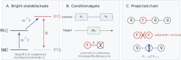
Three consequences of the same interaction shift. The bright state $|W_2\rangle$ is collectively coupled while $|rr\rangle$ is shifted by $B$; a control atom in $|r\rangle$ detunes the target’s nominal $2\pi$ pulse; and strong nearest-neighbor blockade projects a chain flip to $P_{i-1}\sigma_i^xP_{i+1}$.

What breaks the dark-state decomposition

The simple bright and dark states assume equal drive amplitudes and phases. For complex site-dependent couplings $\Omega_i$, the state reached directly from $|gg\rangle$ is instead

$$|B_2\rangle = \frac{ \Omega_1|rg\rangle+\Omega_2|gr\rangle }{ \Omega_{\mathrm{col}} },$$

where

$$\Omega_{\mathrm{col}} = \sqrt{ |\Omega_1|^2+|\Omega_2|^2 }.$$

The orthogonal combination is dark only for the drive Hamiltonian at that instant. Differential detunings, unequal light shifts, motion-dependent phases, and nonidentical interactions can mix bright and dark sectors. Collective enhancement therefore tests spatial mode matching as well as interaction strength.

Finite Blockade

Eliminate the doubly excited state

On single-atom resonance, set $\Delta=0$. If

$$|B| \gg \Omega,$$

the $|rr\rangle$ amplitude follows the bright-state amplitude approximately:

$$c_{rr} \simeq -\frac{\Omega}{\sqrt2\,B} c_W.$$

Substitution gives the leading effective Hamiltonian in $(|gg\rangle,|W_2\rangle)$:

$$\frac{H_{\mathrm{eff}}}{\hbar} \simeq \begin{pmatrix} 0 & \Omega/\sqrt2 \\ \Omega/\sqrt2 & -\Omega^2/(2B) \end{pmatrix}.$$

Finite blockade therefore has two leading consequences:

1. residual double-excitation probability,

   $$P_{rr} \simeq \frac{\Omega^2}{2|B|^2} P_W;$$

2. a coherent bright-state energy shift,

   $$\delta_W \simeq -\frac{\Omega^2}{2B}.$$

The first is leakage; the second is a phase and detuning error. A model that keeps only a hard no-double-excitation rule misses the coherent correction. The sign of $B$ does not affect the leading leakage probability but does reverse the coherent shift.

At nonzero detuning, the energy separation between $|W_2\rangle$ and $|rr\rangle$ is

$$B-\Delta,$$

so the more general leading expressions are

$$\begin{aligned} c_{rr} &\simeq -\frac{\Omega}{\sqrt2(B-\Delta)} c_W, \\ \delta_W &\simeq -\frac{\Omega^2}{2(B-\Delta)}. \end{aligned}$$

The denominator warns against saying “$B\gg\Omega$” without also specifying detuning.

Worked finite-blockade audit

Take

$$\frac{\Omega}{2\pi} = 2.0\ \mathrm{MHz}, \qquad \frac{B}{2\pi} = 40\ \mathrm{MHz}.$$

The ideal collective pi-pulse duration is

$$t_\pi^{(2)} = \frac{\pi}{\sqrt2\,\Omega} \simeq 177\ \mathrm{ns}.$$

At maximum bright-state population, the leakage scale is

$$P_{rr} \simeq \frac12 \left( \frac{2}{40} \right)^2 = 1.25\times10^{-3}.$$

The coherent shift is

$$\frac{\delta_W}{2\pi} \simeq -\frac{(2\ \mathrm{MHz})^2} {2(40\ \mathrm{MHz})} = -50\ \mathrm{kHz}.$$

During the ideal collective pi pulse, this shift accumulates a phase scale

$$|\delta_W|t_\pi^{(2)} \simeq 5.6\times10^{-2}\ \mathrm{rad}.$$

The precise final leakage and phase require solving the three-level Hamiltonian with the actual pulse envelope. The audit nevertheless shows why a small double-excitation probability does not by itself establish a high-fidelity coherent operation.

Multilevel blockade

Real Rydberg pair states form a manifold. If the laser-coupled state overlaps several pair eigenstates $|\mu\rangle$, there is generally no unique scalar $B$. Leakage contains weighted inverse-square energy denominators:

$$P_2 \sim \sum_\mu \frac{ |\kappa_\mu|^2 }{ |\Delta_\mu|^2 },$$

where $\kappa_\mu$ is the coupling to pair eigenstate $\mu$ and $\Delta_\mu$ is its drive-frame energy separation. Weakly shifted channels can dominate even if the mean pair interaction is large.

This is especially important with Zeeman degeneracy, anisotropic $D$ states, or a nearby Förster resonance. A reported blockade strength should state the atomic state, quantization axis, pair orientation, external fields, and how the effective shift was extracted.

Blockade Radius

A family of crossover radii

For a van der Waals interaction

$$V(R) = \frac{C_6}{R^6}, \qquad B(R) = \frac{C_6}{\hbar R^6},$$

a drive-defined blockade radius is often written

$$R_\Omega = \left( \frac{|C_6|} {\hbar\Omega} \right)^{1/6}.$$

This means $|B(R_\Omega)|=\Omega$. It does not mean double excitation is already negligible at $R_\Omega$. In the ideal two-atom estimate, $P_{rr}\sim1/2$ at that equality.

Other legitimate definitions include

$$\begin{aligned} R_\gamma &= \left( \frac{|C_6|} {\hbar\gamma_{\mathrm{exc}}} \right)^{1/6}, \\ R_T &= \left( \frac{|C_6|T} {\hbar} \right)^{1/6}, \end{aligned}$$

where $\gamma_{\mathrm{exc}}$ is an effective excitation linewidth and $1/T$ is a pulse-bandwidth scale. Collective excitation may require comparing $B$ with $\sqrt N\,\Omega$ rather than $\Omega$.

An error-defined radius

If the target is

$$P_{rr} \lesssim \epsilon$$

in the ideal resonant two-atom model, then

$$|B| \gtrsim \frac{\Omega}{\sqrt{2\epsilon}}.$$

The corresponding target-error radius is

$$R_\epsilon = \left[ \frac{ |C_6|\sqrt{2\epsilon} }{ \hbar\Omega } \right]^{1/6}.$$

The weak dependence

$$R_\epsilon \propto \epsilon^{1/12}$$

means that a much stricter leakage target reduces the radius only gradually. It also means a single significant digit in a quoted radius can hide a large change in the implied error.

Numerical comparison

Consider an illustrative isotropic coefficient

$$\frac{|C_6|}{h} = 1.0\ \mathrm{THz}\,\mu\mathrm m^6$$

and $\Omega/(2\pi)=2.0\ \mathrm{MHz}$. Because both $B$ and $\Omega$ may be compared in angular-frequency units, the same ratio can be evaluated using $|C_6|/h$ and ordinary frequencies.

Definition	Comparison scale in ordinary frequency	Radius
drive equality, $	B	=\Omega$
spectral width example	$10\ \mathrm{MHz}$	$6.81\ \mu\mathrm m$
$P_{rr}\lesssim10^{-3}$ ideal target	$44.7\ \mathrm{MHz}$	$5.31\ \mu\mathrm m$

The conventional drive-equality radius is therefore almost seventy percent larger than the radius associated with a $10^{-3}$ leakage target. Neither number is wrong; they answer different questions.

Angular and statistical radii

If $C_6=C_6(\theta,\phi)$, then

$$R_b = R_b(\theta,\phi).$$

The blockade region need not be circular or spherical. Position uncertainty also makes $B$ a random variable. For $V\propto R^{-6}$,

$$\frac{\delta B}{B} \simeq -6\frac{\delta R}{R},$$

so the tails of the position distribution can dominate rare double excitations.

For a general comparison scale $S$,

$$R_b = \left( \frac{|C_6|}{\hbar S} \right)^{1/6},$$

and small independent calibration shifts obey

$$\frac{\delta R_b}{R_b} \simeq \frac16 \left( \frac{\delta |C_6|}{|C_6|} -\frac{\delta S}{S} \right).$$

The sixth root makes the radius numerically robust while the blockade error, which depends roughly on $B^{-2}$, remains much more sensitive.

Blockade, Facilitation, and Pair Resonance

The rotating-frame energies of the one- and two-excitation sectors are

$$E_W = -\hbar\Delta, \qquad E_{rr} = \hbar(B-2\Delta).$$

Three conditions answer different questions:

Condition	Interpretation
$	B-\Delta
$B\simeq\Delta$	adding a second excitation next to an existing Rydberg excitation is resonant; facilitation condition
$B\simeq2\Delta$	$

Thus a large bare $|B|$ does not guarantee blockade under every detuned protocol. Detuning can compensate the interaction. Deliberately using such a condition is called facilitation or antiblockade in different contexts; the name should be accompanied by the actual resonance condition.

The sign matters. Repulsive and attractive pair shifts move resonances in opposite detuning directions. A scan that measures only the magnitude of double-excitation suppression can miss this information, while spectroscopy retains it.

Collective Excitation and Superatoms

N uniformly driven atoms

For $N$ atoms initially in

$$|G\rangle = |g_1g_2\cdots g_N\rangle,$$

define the symmetric one-excitation state

$$|W_N\rangle = \frac{1}{\sqrt N} \sum_{i=1}^{N} |g_1\cdots r_i\cdots g_N\rangle.$$

The uniform drive

$$H_d = \frac{\hbar\Omega}{2} \sum_i \left( |r_i\rangle\langle g_i| + \mathrm{h.c.} \right)$$

has matrix element

$$\langle W_N|H_d|G\rangle = \frac{\hbar\sqrt N\,\Omega}{2}.$$

If every doubly excited state is sufficiently detuned, the ensemble behaves as a two-state system with collective Rabi frequency

$$\Omega_N = \sqrt N\,\Omega.$$

This is the superatom limit. The single Rydberg excitation is shared coherently among the atoms. It is not correct to say that one unknown atom was excited unless a measurement localizes the excitation.

Phase-matched collective state

If the laser phase at site $i$ is $\phi_i$, the bright state is

$$|W_{\boldsymbol\phi}\rangle = \frac{1}{\sqrt N} \sum_i e^{i\phi_i} |g_1\cdots r_i\cdots g_N\rangle.$$

For spatial phase $\phi_i=\mathbf k_{\mathrm{eff}}\cdot\mathbf r_i$, motion dephases the collective spin wave. De-excitation into a selected optical mode also depends on this phase pattern. The state is symmetric in population but not necessarily in optical phase.

For nonuniform couplings, replace $\sqrt N\,\Omega$ by

$$\Omega_{\mathrm{col}} = \sqrt{ \sum_i|\Omega_i|^2 },$$

and weight the bright state by $\Omega_i$. Inferring atom number from a measured collective Rabi frequency is valid only after coupling inhomogeneity is bounded.

Finite blockade in an ensemble

Let $B_{ij}$ be the interaction shift of the doubly excited pair $ij$. Starting from a normalized symmetric one-excitation state, the coupling to that pair is $\Omega/\sqrt N$. In the simplest nondegenerate, resonant elimination,

$$P_2 \simeq \frac{\Omega^2}{N} \sum_{i<j} \frac{1}{|B_{ij}|^2} P_W.$$

Define a harmonic-type effective blockade shift by

$$\frac{1}{B_{\mathrm{eff}}^2} = \frac{2}{N(N-1)} \sum_{i<j} \frac{1}{|B_{ij}|^2}.$$

Then

$$P_2 \simeq \frac{N-1}{2} \frac{\Omega^2}{B_{\mathrm{eff}}^2} P_W.$$

For uniform $B_{ij}=B$, this reduces to

$$P_2 \simeq \frac{N-1}{2} \left( \frac{\Omega}{B} \right)^2 P_W.$$

The sum weights weakly blockaded pairs strongly. Increasing atom number at fixed geometry and drive can therefore worsen leakage even while the desired collective coupling grows as $\sqrt N$.

The formula assumes independent pair eigenstates and weak admixture. Pair state mixing, anisotropy, nonuniform drive, and several-excitation pathways require the full multilevel Hamiltonian.

How Blockade Is Measured

Suppression of double excitation

The most direct observable is the corrected probability $P_{rr}$ for both atoms to be excited. Compare it with the independent-atom expectation using the same pulse. A small raw double-loss fraction is not enough because a loss-based detector can misclassify $|rr\rangle$, ordinary loss, or failed recapture.

The readout matrix should be calibrated for all relevant two-atom outcomes:

$$\left( gg,\, gr,\, rg,\, rr,\, \text{loss or leakage} \right).$$

Independent single-site corrections can fail if ionization, recapture, or imaging errors are correlated.

Collective enhancement

On resonance, compare the single-atom oscillation frequency $\Omega$ with the pair bright-state frequency $\sqrt2\,\Omega$. Seeing both collective enhancement and suppressed $P_{rr}$ is stronger evidence than either alone: the first tests coherent symmetry, while the second tests interaction detuning.

Interaction-shifted spectroscopy

Frequency scans can resolve the shifted pair resonance or bound its absence. Varying separation and orientation tests whether the extracted shift follows the intended pair potential. A scalar $R^{-6}$ fit should be compared with a multilevel pair-state calculation when angular or field dependence is appreciable.

Distance sweep and model fit

A blockade-radius measurement should fit a smooth finite-$B$ model to $P_{rr}(R)$ rather than thresholding the data into blocked and unblocked points. The report should include

• the radius definition;
• pulse duration, detuning, and linewidth;
• calibrated position uncertainty;
• readout correction and confidence interval;
• pair orientation and external fields; and
• model alternatives or residuals.

Controls

Useful controls change one ingredient at a time:

• excite only one atom;
• move the atoms farther apart;
• select a more weakly interacting Rydberg state;
• reverse or vary detuning;
• rotate the pair relative to the quantization axis; and
• scan the electric field across a pair resonance.

These distinguish blockade from technical suppression caused by reduced laser intensity, misalignment, or state-preparation errors.

Two-Qubit Gates

Conditional dynamics

Encode qubits in long-lived states $|0\rangle$ and $|1\rangle$, and couple only $|1\rangle$ to $|r\rangle$. A standard conceptual sequence is

$$\pi_{\mathrm c} \longrightarrow 2\pi_{\mathrm t} \longrightarrow \pi_{\mathrm c},$$

where c and t label control and target.

1. The first control pi pulse maps $|1\rangle_{\mathrm c}\leftrightarrow|r\rangle_{\mathrm c}$.
2. If the control is not Rydberg excited, a target $2\pi$ pulse executes a closed Rabi cycle and contributes a phase.
3. If the control occupies $|r\rangle$, the interaction shifts the target’s doubly excited state and suppresses that cycle.
4. The final control pi pulse returns population to the computational subspace.

For one simple pulse-phase convention, the computational basis transforms as

$$\begin{aligned} |00\rangle&\longmapsto |00\rangle, \\ |01\rangle&\longmapsto-|01\rangle, \\ |10\rangle&\longmapsto-|10\rangle, \\ |11\rangle&\longmapsto-|11\rangle. \end{aligned}$$

The diagonal unitary

$$U = \operatorname{diag}(1,-1,-1,-1)$$

is locally equivalent to a controlled-$Z$ gate. Its gauge-invariant two-qubit phase is

$$\Phi_{\mathrm{ent}} = \phi_{00}-\phi_{01}-\phi_{10}+\phi_{11} = \pi \pmod{2\pi}.$$

Single-qubit phase corrections convert it to the usual $\operatorname{diag}(1,1,1,-1)$ convention. Actual pulse phases and level shifts must be tracked; population return alone does not establish the entangling phase.

Beyond the three-pulse picture

Modern blockade gates can use global symmetric pulses, time-dependent phase or detuning, dark-state paths, adiabatic dressing, optimal control, or direct multi-qubit protocols. These methods redistribute time spent in lossy states and sensitivity to calibration errors. The three-pulse sequence remains a clear mechanism, not a universal optimum.

Intrinsic trade-off

A useful schematic error model is

$$\epsilon(\Omega) \simeq \frac{a}{\Omega\tau_r} + b\left( \frac{\Omega}{B} \right)^2,$$

where $\tau_r$ is the Rydberg lifetime and $a,b$ depend on the pulse protocol. Driving faster reduces time exposed to decay but worsens finite-blockade error. Minimization gives the scaling

$$\Omega_{\mathrm{opt}} \propto \left( \frac{B^2}{\tau_r} \right)^{1/3}, \qquad \epsilon_{\mathrm{opt}} \propto (B\tau_r)^{-2/3}.$$

This is not a complete experimental error budget. Intermediate-state scattering, Doppler shifts, laser phase and intensity noise, adjacent Rydberg levels, pulse rise time, differential light shifts, addressing crosstalk, motion, and readout can dominate.

What constitutes gate evidence

Different measurements support different claims.

Measurement	What it establishes	What it does not establish alone
truth table	basis-state population transfer	coherent phase or action on superpositions
Bell-state populations and parity	entanglement-generation fidelity or lower bound	average fidelity of an arbitrary gate input
process tomography	reconstructed process under model assumptions	scalable, drift-robust average performance
repeated-gate or randomized protocol	per-gate decay metric over a sampled ensemble	every coherent and leakage mechanism separately
leakage or erasure detection	probability and location of detectable failures	unconditional success when failed shots are discarded

A conditional Bell-state fidelity after erasure excision and an unconditional average gate fidelity are both useful, but they are not interchangeable. Similarly, correcting state-preparation-and-measurement errors can isolate an operation estimate, but the correction model and uncertainty must be stated.

Blockade in Quantum Simulation

Soft-interaction Hamiltonian

The calibrated array begins with

$$\frac{H}{\hbar} = \frac{\Omega}{2} \sum_i\sigma_i^x -\Delta\sum_i n_i + \sum_{i<j}B_{ij}n_i n_j.$$

This is a soft constraint: doubly excited configurations remain in the Hilbert space but cost interaction energy. The full long-range $B_{ij}$ tail can influence phase boundaries and dynamics even when nearest neighbors are strongly blockaded.

Projected nearest-neighbor limit

In a one-dimensional chain with

$$|B_{i,i+1}| \gg \Omega,\ |\Delta|,$$

project onto the subspace with no adjacent Rydberg excitations. Define

$$P_i = 1-n_i = |g_i\rangle\langle g_i|.$$

A site may flip only if both neighbors are in $|g\rangle$, giving

$$\frac{H_{\mathrm{PXP}}}{\hbar} = \frac{\Omega}{2} \sum_i P_{i-1}\sigma_i^xP_{i+1} -\Delta\sum_i n_i.$$

At $\Delta=0$, the name PXP refers to the projector–flip–projector structure. Boundary terms contain only the available neighbor projector. This Hamiltonian describes constrained dynamics and underlies the connection between Rydberg chains and quantum many-body scars.

Finite blockade produces leakage and virtual corrections of order

$$\frac{\Omega}{B_{\mathrm{nn}}} \quad\text{and}\quad \frac{\Omega^2}{B_{\mathrm{nn}}},$$

while next-neighbor interactions remain explicit. The controlled derivation can be organized with a projection or Schrieffer–Wolff transformation.

Blockade graphs and independent sets

Construct a graph whose vertices are atoms and whose edges connect pairs treated as mutually blockaded. In the hard-constraint idealization, an allowed Rydberg configuration is an independent set: no occupied vertices share an edge.

For positive detuning in the convention used here, the term

$$-\hbar\Delta\sum_i n_i$$

favors more Rydberg excitations. In an ideal hard-constraint endpoint, the lowest-energy configurations maximize the number of occupied, mutually nonadjacent vertices. This gives the hardware-efficient connection to the maximum-independent-set problem.

The graph itself is model-dependent. A finite, anisotropic interaction does not create a sharp edge, and interactions beyond chosen edges shift different independent sets unequally. Claims about optimization performance must include the soft interaction Hamiltonian, preparation schedule, readout correction, and classical comparison protocol.

Ordered phases and nonequilibrium dynamics

Blockade plus detuning can favor spatially ordered Rydberg patterns. Quenches from special product states can show long-lived revivals described by constrained models. These phenomena are applications of the blockade Hamiltonian, not additional evidence that blockade is perfect.

The many-body interpretation belongs to Transverse-Field Ising Model and related many-body pages. Here the experimental responsibility is to show that the projected model and its corrections follow from independently calibrated $\Omega_i$, $\Delta_i$, $B_{ij}$, positions, and noise channels.

Validity and Error Ledger

Atomic and pair-state validity

• Is the selected pair eigenstate spectrally isolated?
• Are Zeeman and hyperfine channels retained where needed?
• Is the $C_6/R^6$ approximation valid over the sampled distances?
• Are electric-field drift and pair orientation measured?
• Does the multipole approximation remain valid?

Drive validity

• Are rotating-wave and two-level reductions controlled?
• Are single-atom light shifts and intermediate-state scattering included?
• Are $\Omega_i$, optical phases, and pulse transients measured?
• Is the denominator $B-\Delta$ large throughout the pulse?
• Are adjacent Rydberg states or dark states populated?

Motional validity

• Is the position distribution narrow enough for the desired $B_{ij}$?
• Is Doppler dephasing small on the operation timescale?
• Are tweezers on, off, or state insensitive during excitation?
• Does interaction-induced force entangle motion and internal state?
• Are recapture and loss separated from Rydberg population?

Measurement validity

• Is double excitation distinguished from two-atom loss?
• Are confusion-matrix uncertainties propagated?
• Are errors correlated across sites?
• Is postselection reported with its acceptance probability?
• Are Bell-state, process, and average gate fidelities labeled correctly?

Many-body validity

• Does every forbidden edge satisfy the chosen error criterion?
• Are beyond-edge interaction tails included?
• Are finite-blockade virtual shifts retained or bounded?
• Does small-system data close with independently calibrated parameters?
• Are observable uncertainties compared with model discrepancies?

Common Mistakes

Treating the blockade radius as a wall

The interaction and double-excitation probability vary smoothly with distance. A radius is a convention-dependent crossover.

Defining the radius without a comparison scale

$|C_6|$ and $R$ alone do not define blockade. One must state the drive, linewidth, pulse bandwidth, collective scale, or target error.

Equating B much greater than Omega with zero error

Finite blockade leaves both leakage of order $(\Omega/B)^2$ and a coherent shift of order $\Omega^2/B$.

Forgetting detuning in the blockade denominator

The one-to-two-excitation separation is $B-\Delta$. A detuned drive can facilitate rather than suppress a second excitation.

Averaging over pair interactions

Leakage weights weak shifts through inverse-square denominators. A weak angular channel can dominate the mean interaction.

Calling every sqrt-N oscillation a superatom

The $\sqrt N$ law assumes coherent phase matching and known coupling uniformity. Fluctuating atom number or $\Omega_i$ can mimic damping and shift the apparent frequency.

Using raw loss as double-excitation probability

Loss-based detection confounds Rydberg population, background loss, failed recapture, and leakage. A calibrated multi-outcome readout model is required.

Calling a truth table a coherent gate characterization

A truth table does not measure relative phases. A diagonal operation can have the right basis populations and the wrong entangling phase.

Calling Bell-state fidelity gate fidelity

Bell-state generation includes preparation, single-qubit operations, the entangling operation, and readout. It samples one input and one target state, not the average gate action.

Treating the PXP model as the exact apparatus Hamiltonian

PXP is a projected limit. Finite blockade, long-range tails, motion, loss, and inhomogeneous parameters remain physical corrections.

Exercises

Exercise 1: Derive the bright-sector Hamiltonian

Starting from the four-state two-atom Hamiltonian, transform to the basis

$$\left( |gg\rangle,\, |W_2\rangle,\, |D_2\rangle,\, |rr\rangle \right).$$

Show that $|D_2\rangle$ decouples under uniform driving and derive the three-state bright-sector Hamiltonian.

Solution

The laser couples

$$H_d|gg\rangle = \frac{\hbar\Omega}{2} \left( |gr\rangle+|rg\rangle \right) = \frac{\hbar\Omega}{\sqrt2} |W_2\rangle.$$

Similarly,

$$H_d|W_2\rangle = \frac{\hbar\Omega}{\sqrt2} \left( |gg\rangle+|rr\rangle \right),$$

whereas

$$H_d|D_2\rangle = 0.$$

The detuning gives energy $-\hbar\Delta$ to both one-excitation states and $-2\hbar\Delta$ to $|rr\rangle$. The interaction adds $\hbar B$ only to $|rr\rangle$. Therefore

$$\frac{H}{\hbar} = \begin{pmatrix} 0 & \Omega/\sqrt2 & 0 & 0 \\ \Omega/\sqrt2 & -\Delta & 0 & \Omega/\sqrt2 \\ 0 & 0 & -\Delta & 0 \\ 0 & \Omega/\sqrt2 & 0 & -2\Delta+B \end{pmatrix}.$$

Removing the isolated dark-state row and column gives

$$\frac{H_{\mathrm{bright}}}{\hbar} = \begin{pmatrix} 0 & \Omega/\sqrt2 & 0 \\ \Omega/\sqrt2 & -\Delta & \Omega/\sqrt2 \\ 0 & \Omega/\sqrt2 & -2\Delta+B \end{pmatrix}.$$

Exercise 2: Leakage and coherent shift

On resonance, eliminate $|rr\rangle$ to leading order in $\Omega/B$. Derive the bright-state shift and the maximum double-excitation scale. Evaluate both for

$$\frac{\Omega}{2\pi}=2.0\ \mathrm{MHz}, \qquad \frac{B}{2\pi}=40\ \mathrm{MHz}.$$

Also calculate the ideal collective pi-pulse duration.

Solution

The $|rr\rangle$ equation is

$$i\dot c_{rr} = \frac{\Omega}{\sqrt2}c_W +Bc_{rr}.$$

For $|B|\gg\Omega$, set $\dot c_{rr}\simeq0$:

$$c_{rr} \simeq -\frac{\Omega}{\sqrt2 B}c_W.$$

Substitution into the $c_W$ equation gives

$$\delta_W = -\frac{\Omega^2}{2B}.$$

At $P_W\simeq1$,

$$P_{rr} \simeq \frac{\Omega^2}{2B^2} = \frac12 \left( \frac{2}{40} \right)^2 = 1.25\times10^{-3}.$$

The shift is

$$\frac{\delta_W}{2\pi} = -\frac{(2\ \mathrm{MHz})^2} {2(40\ \mathrm{MHz})} = -50\ \mathrm{kHz}.$$

The collective Rabi frequency is $\sqrt2\,\Omega$, so

$$t_\pi^{(2)} = \frac{\pi}{\sqrt2\,\Omega} = \frac{1}{2\sqrt2(2.0\ \mathrm{MHz})} \simeq 177\ \mathrm{ns}.$$

Exercise 3: Three blockade radii

Take

$$\frac{|C_6|}{h} = 1.0\ \mathrm{THz}\,\mu\mathrm m^6, \qquad \frac{\Omega}{2\pi} = 2.0\ \mathrm{MHz}.$$

Calculate:

1. the drive-equality radius $R_\Omega$;
2. the radius obtained with a $10\ \mathrm{MHz}$ excitation-width scale;
3. the ideal target-error radius for $P_{rr}\leq10^{-3}$.

Explain why the three answers can all be valid.

Solution

Using ordinary-frequency quantities,

$$R = \left[ \frac{|C_6|/h}{S/(2\pi)} \right]^{1/6}.$$

For the drive equality,

$$R_\Omega = \left( \frac{10^{12}}{2.0\times10^6} \right)^{1/6} \mu\mathrm m \simeq 8.91\ \mu\mathrm m.$$

For a $10\ \mathrm{MHz}$ width,

$$R_\gamma = \left( \frac{10^{12}}{10^7} \right)^{1/6} \mu\mathrm m \simeq 6.81\ \mu\mathrm m.$$

The leakage target requires

$$\frac{|B|}{\Omega} \geq \frac{1}{\sqrt{2\times10^{-3}}} \simeq 22.36.$$

Thus the interaction-frequency scale is

$$(22.36)(2.0\ \mathrm{MHz}) = 44.7\ \mathrm{MHz},$$

and

$$R_\epsilon = \left( \frac{10^{12}}{44.7\times10^6} \right)^{1/6} \mu\mathrm m \simeq 5.31\ \mu\mathrm m.$$

The definitions compare the same interaction with different physical scales: coherent drive, spectral resolution, and a specified leakage target.

Exercise 4: N-atom collective coupling and leakage

For $N$ uniformly driven atoms:

1. derive the coupling between $|G\rangle$ and $|W_N\rangle$;
2. show that the collective Rabi frequency is $\sqrt N\,\Omega$;
3. assume every pair has the same blockade shift $B$ and derive the leading total double-excitation probability at $P_W=1$.

For $N=10$ and $B/\Omega=50$, estimate $P_2$.

Solution

Acting on the collective ground state,

$$H_d|G\rangle = \frac{\hbar\Omega}{2} \sum_i|i\rangle = \frac{\hbar\sqrt N\,\Omega}{2} |W_N\rangle.$$

Therefore

$$\Omega_N = \sqrt N\,\Omega.$$

For a particular double excitation $|ij\rangle$, there are two paths from $|W_N\rangle$, one from its $|i\rangle$ component and one from its $|j\rangle$ component. Their total matrix element is

$$\frac{\hbar\Omega}{\sqrt N}.$$

Elimination gives probability

$$\frac{\Omega^2}{NB^2}$$

in each of the $N(N-1)/2$ pair states. Hence

$$P_2 \simeq \frac{N-1}{2} \left( \frac{\Omega}{B} \right)^2.$$

For $N=10$ and $B/\Omega=50$,

$$P_2 \simeq \frac{9}{2(50)^2} = 1.8\times10^{-3}.$$

This estimate assumes equal nondegenerate pair shifts and no coupling among the double-excitation states.

Exercise 5: Blockade or facilitation?

For the two-atom Hamiltonian with detuning $\Delta$:

1. find the energy cost for adding a second Rydberg excitation when one is already present;
2. find the condition for $|gg\rangle$ and $|rr\rangle$ to be degenerate in the rotating frame;
3. evaluate both conditions for $B/(2\pi)=30\ \mathrm{MHz}$.

Solution

The one-excitation energy is

$$E_W = -\hbar\Delta,$$

and the double-excitation energy is

$$E_{rr} = \hbar(B-2\Delta).$$

Adding the second excitation costs

$$E_{rr}-E_W = \hbar(B-\Delta).$$

It is resonant when

$$\Delta \simeq B.$$

The pair state is degenerate with $|gg\rangle$ when

$$B-2\Delta = 0,$$

or

$$\Delta \simeq \frac{B}{2}.$$

For $B/(2\pi)=30\ \mathrm{MHz}$, the facilitation condition for adding a second excitation is $\Delta/(2\pi)\simeq30\ \mathrm{MHz}$, while the two-photon pair-resonance condition is $\Delta/(2\pi)\simeq15\ \mathrm{MHz}$.

Exercise 6: Entangling phase of the three-pulse gate

Assume the blockade-gate sequence produces

$$U = \operatorname{diag}(1,-1,-1,-1)$$

in the ordered basis $(|00\rangle,|01\rangle,|10\rangle,|11\rangle)$.

1. Calculate the entangling phase $\Phi_{\mathrm{ent}} =\phi_{00}-\phi_{01}-\phi_{10}+\phi_{11}$.
2. Find local $Z$ operations that convert $U$ to $\operatorname{diag}(1,1,1,-1)$.
3. Explain why a truth-table measurement would not determine $\Phi_{\mathrm{ent}}$.

Solution

Choose phases

$$(\phi_{00},\phi_{01},\phi_{10},\phi_{11}) = (0,\pi,\pi,\pi).$$

Then

$$\Phi_{\mathrm{ent}} = 0-\pi-\pi+\pi = -\pi \equiv \pi \pmod{2\pi}.$$

Apply $Z$ to both qubits:

$$(Z\otimes Z)U = \operatorname{diag}(1,1,1,-1).$$

A truth table records only output populations for computational-basis inputs. Every diagonal unitary has the identity truth table, regardless of its relative phases. Superposition inputs and phase-sensitive measurements are required.

Exercise 7: Optimize a schematic gate error

Let

$$\epsilon(\Omega) = \frac{a}{\Omega\tau} + b\frac{\Omega^2}{B^2},$$

with $a,b>0$. Find $\Omega_{\mathrm{opt}}$ and show that the optimized error scales as $(B\tau)^{-2/3}$. At the optimum, what is the ratio of the lifetime term to the blockade term?

Solution

Differentiate:

$$\frac{d\epsilon}{d\Omega} = -\frac{a}{\Omega^2\tau} + \frac{2b\Omega}{B^2}.$$

Setting this to zero gives

$$\Omega_{\mathrm{opt}}^3 = \frac{aB^2}{2b\tau},$$

or

$$\Omega_{\mathrm{opt}} = \left( \frac{aB^2}{2b\tau} \right)^{1/3}.$$

Substitution shows that both terms scale as

$$(B\tau)^{-2/3},$$

so

$$\epsilon_{\mathrm{opt}} \propto (B\tau)^{-2/3}.$$

The stationarity equation may be rearranged as

$$\frac{a}{\Omega_{\mathrm{opt}}\tau} = 2b \frac{\Omega_{\mathrm{opt}}^2}{B^2}.$$

Thus the lifetime contribution is twice the blockade contribution in this particular two-term model.

Exercise 8: Derive and test the PXP limit

Consider a one-dimensional chain with nearest-neighbor interaction $B_{\mathrm{nn}}$ much larger than $\Omega$ and $|\Delta|$.

1. Project the drive onto the subspace with no adjacent Rydberg excitations and derive the PXP Hamiltonian.
2. List three leading corrections in a real array.
3. Design a small-system validation test that distinguishes the projected model from the full soft-interaction model.

Solution

Let

$$P_i = |g_i\rangle\langle g_i| = 1-n_i.$$

Within the constrained subspace, flipping site $i$ is allowed only when its neighbors are both in $|g\rangle$. Therefore

$$\frac{H_{\mathrm{PXP}}}{\hbar} = \frac{\Omega}{2} \sum_i P_{i-1}\sigma_i^xP_{i+1} -\Delta\sum_i n_i,$$

with one projector at an open boundary.

Leading corrections include:

• real population leakage into adjacent-excitation states, of amplitude scale $\Omega/B_{\mathrm{nn}}$;
• virtual energy and coupling corrections of scale $\Omega^2/B_{\mathrm{nn}}$;
• explicit next-neighbor and longer-range interactions;
• site-dependent $\Omega_i$ and $\Delta_i$;
• decay, dephasing, motion, and readout errors.

A useful validation test prepares all basis states of a three- or four-atom chain, measures short-time transition probabilities, and compares predictions using independently calibrated $\Omega$, $\Delta$, and $B_{ij}$. States with an excited neighbor directly test forbidden flips, while states without one test the allowed collective drive. Sweeping $\Omega/B_{\mathrm{nn}}$ reveals whether deviations follow the expected leakage and virtual-shift scaling.

References

1. D. Jaksch, J. I. Cirac, P. Zoller, S. L. Rolston, R. Côté, and M. D. Lukin, “Fast quantum gates for neutral atoms,” Physical Review Letters 85, 2208–2211 (2000), doi:10.1103/PhysRevLett.85.2208.
2. M. D. Lukin, M. Fleischhauer, R. Côté, L. M. Duan, D. Jaksch, J. I. Cirac, and P. Zoller, “Dipole blockade and quantum information processing in mesoscopic atomic ensembles,” Physical Review Letters 87, 037901 (2001), doi:10.1103/PhysRevLett.87.037901.
3. T. G. Walker and M. Saffman, “Consequences of Zeeman degeneracy for the van der Waals blockade between Rydberg atoms,” Physical Review A 77, 032723 (2008), doi:10.1103/PhysRevA.77.032723.
4. E. Urban et al., “Observation of Rydberg blockade between two atoms,” Nature Physics 5, 110–114 (2009), doi:10.1038/nphys1178.
5. A. Gaëtan et al., “Observation of collective excitation of two individual atoms in the Rydberg blockade regime,” Nature Physics 5, 115–118 (2009), doi:10.1038/nphys1183.
6. M. Saffman, T. G. Walker, and K. Mølmer, “Quantum information with Rydberg atoms,” Reviews of Modern Physics 82, 2313–2363 (2010), doi:10.1103/RevModPhys.82.2313.
7. T. Wilk et al., “Entanglement of two individual neutral atoms using Rydberg blockade,” Physical Review Letters 104, 010502 (2010), doi:10.1103/PhysRevLett.104.010502.
8. L. Isenhower et al., “Demonstration of a neutral atom controlled-NOT quantum gate,” Physical Review Letters 104, 010503 (2010), doi:10.1103/PhysRevLett.104.010503.
9. X. L. Zhang, L. Isenhower, A. T. Gill, T. G. Walker, and M. Saffman, “Fidelity of a Rydberg-blockade quantum gate from simulated quantum process tomography,” Physical Review A 85, 042310 (2012), doi:10.1103/PhysRevA.85.042310.
10. H. Labuhn et al., “Tunable two-dimensional arrays of single Rydberg atoms for realizing quantum Ising models,” Nature 534, 667–670 (2016), doi:10.1038/nature18274.
11. H. Bernien et al., “Probing many-body dynamics on a 51-atom quantum simulator,” Nature 551, 579–584 (2017), doi:10.1038/nature24622.
12. C. J. Turner, A. A. Michailidis, D. A. Abanin, M. Serbyn, and Z. Papić, “Weak ergodicity breaking from quantum many-body scars,” Nature Physics 14, 745–749 (2018), doi:10.1038/s41567-018-0137-5.
13. H. Levine et al., “High-fidelity control and entanglement of Rydberg-atom qubits,” Physical Review Letters 121, 123603 (2018), doi:10.1103/PhysRevLett.121.123603.
14. H. Levine et al., “Parallel implementation of high-fidelity multiqubit gates with neutral atoms,” Physical Review Letters 123, 170503 (2019), doi:10.1103/PhysRevLett.123.170503.
15. T. M. Graham et al., “Rydberg-mediated entanglement in a two-dimensional neutral atom qubit array,” Physical Review Letters 123, 230501 (2019), doi:10.1103/PhysRevLett.123.230501.
16. I. S. Madjarov et al., “High-fidelity entanglement and detection of alkaline-earth Rydberg atoms,” Nature Physics 16, 857–861 (2020), doi:10.1038/s41567-020-0903-z.
17. S. Ebadi et al., “Quantum optimization of maximum independent set using Rydberg atom arrays,” Science 376, 1209–1215 (2022), doi:10.1126/science.abo6587.
18. P. Scholl et al., “Erasure conversion in a high-fidelity Rydberg quantum simulator,” Nature 622, 273–278 (2023), doi:10.1038/s41586-023-06516-4.
19. S. J. Evered et al., “High-fidelity parallel entangling gates on a neutral-atom quantum computer,” Nature 622, 268–272 (2023), doi:10.1038/s41586-023-06481-y.
20. P. Fendley, K. Sengupta, and S. Sachdev, “Competing density-wave orders in a one-dimensional hard-boson model,” Physical Review B 69, 075106 (2004), doi:10.1103/PhysRevB.69.075106.

Cross-Links

• Neutral-Atom and Rydberg Qubits places blockade gates and constrained interactions inside the complete loading, routing, readout, throughput, and error-correction architecture.
• Rydberg Array Frontiers tracks current array scale, gate and logical benchmarks, analog many-body results, erasure-aware architectures, and optimization evidence.
• Rydberg Atoms develops the excitation, trapping, field-control, detection, and calibration stack needed before applying the blockade model.
• Rydberg Atoms Basics derives the atomic scaling and pair-interaction mechanisms summarized by $B$ here.
• Optical Tweezers develops the position control and readout pipeline for configurable arrays.
• Neutral Atoms treats decay, dephasing, atom loss, and measurement channels in open-system language.
• Bell States develops the entangled targets used in blockade-gate demonstrations.
• Transverse-Field Ising Model develops a canonical many-body model realized in Rydberg-array regimes.
• Quantum Information Roadmap connects gate metrics, entanglement, channels, and error correction.