Atom Interferometry

An atom interferometer coherently splits an atomic center-of-mass amplitude, lets the alternatives accumulate phase, and recombines them so that phase appears in measured populations or positions. The splitter can be a material grating, a standing optical wave, a two-photon Raman pulse, a Bragg pulse, a magnetic potential, or a guided-atom junction. The most widely used inertial configuration is the three-pulse light-pulse interferometer:

$$\frac{\pi}{2} \;-\; T \;-\; \pi \;-\; T \;-\; \frac{\pi}{2}.$$

The first pulse creates two momentum alternatives, the middle pulse redirects them, and the last pulse recombines them. For ideal instantaneous pulses and uniform acceleration,

$$\Phi_a = \mathbf k_{\mathrm{eff}} \mathbin{\cdot} \mathbf a\,T^2$$

in the convention used here. This compact formula is not the whole experiment. Its use requires a phase reference carried by the laser fields, controlled internal states, closed wave packets, known pulse timing, measured contrast, calibrated detection, and an account of vibration, rotation, wavefront, magnetic, optical, and gravity-gradient effects.

Atom interferometry is therefore both matter-wave physics and precision control. The atoms provide freely evolving quantum test masses; the light pulses provide beam splitters, mirrors, clocks, and rulers.

Canonical Scope

Interference With Matter owns the historical and conceptual survey from electrons and neutrons to atoms and molecules. Interferometry owns the cross-platform instrument logic. Optical Interferometers owns the two-mode optical Mach–Zehnder transformation, photon statistics, shot-noise baseline, and squeezed-light enhancement.

Ramsey Interferometry owns separated-pulse interference between internal states when no spatially separated center-of-mass paths are required. Quantum Sensing owns the general estimator, Fisher-information, resource, and decoherence-limited sensing framework.

This page owns:

• coherent atom-optical beam splitters and mirrors;
• Raman and Bragg momentum transfer;
• the three-pulse light-pulse Mach–Zehnder sequence;
• propagation, laser, internal, and separation phase bookkeeping;
• the acceleration and rotation transfer functions;
• sensitivity functions for time-dependent inertial signals;
• wave-packet closure, overlap, and contrast;
• state-selective readout and phase estimation;
• the platform-level noise and calibration ledger; and
• an introductory map to gravimetry, gradiometry, gyroscopy, and inertial sensing.

Detailed sensor uncertainty budgets and application-specific metrology are developed in Atom-Interferometric Sensors rather than duplicated in the interferometer derivation here. Gravimetry and Inertial Sensing owns the matched independent-atom benchmark, squeezed-state transfer, information-rate accounting, and evidence required for a quantum-enhanced inertial estimate.

Conventions

Let a Raman process absorb from field 1 and stimulate emission into field 2. Define

$$\mathbf k_{\mathrm{eff}} = \mathbf k_1-\mathbf k_2,$$

and let a successful transition transfer momentum

$$\Delta\mathbf p = \hbar\mathbf k_{\mathrm{eff}}.$$

The effective optical phase is

$$\phi_L(\mathbf r,t) = \mathbf k_{\mathrm{eff}} \mathbin{\cdot} \mathbf r - \varphi(t),$$

where $\varphi(t)$ contains the microwave or optical frequency-difference phase synthesized by the laser system. A different sign convention for $\phi_L$ reverses several formulas together but cannot change a measured probability.

For the ideal three-pulse sequence, pulse centers occur at

$$t_1=0, \qquad t_2=T, \qquad t_3=2T.$$

The acceleration $\mathbf a$ means acceleration of the atoms relative to the optical phase fronts. Motion of a retroreflection mirror therefore enters the same observable as atomic acceleration, with the appropriate opposite relative sign.

The ideal output model is written

$$P_e = P_0 + \frac{C}{2} \cos \left( \Phi+\phi_{\mathrm{off}} \right),$$

where $P_0$ is an offset, $C$ is contrast, and $\phi_{\mathrm{off}}$ collects a controlled analysis phase and stable biases. An ideal balanced two-port interferometer has $P_0=1/2$ and $C=1$.

Matter Waves and Interferometer Phase

Center-of-mass phase

For a nonrelativistic center-of-mass path $\mathbf r(t)$ with Lagrangian $L$, the propagation amplitude carries phase

$$\phi_{\mathrm{prop}} = \frac{S}{\hbar}, \qquad S = \int L \left( \mathbf r,\dot{\mathbf r},t \right) dt.$$

Two alternatives can interfere only when the final measurement does not retain information that distinguishes them. Their propagation contribution is

$$\Delta\phi_{\mathrm{prop}} = \frac{S_u-S_\ell}{\hbar}.$$

This action language is universal, but a light-pulse atom interferometer also receives phases at each atom–light interaction. The observed phase is not generally just a classical action difference.

Complete phase ledger

A useful decomposition is

$$\Phi = \Phi_{\mathrm{prop}} + \Phi_{\mathrm{laser}} + \Phi_{\mathrm{int}} + \Phi_{\mathrm{sep}}.$$

The terms are:

• $\Phi_{\mathrm{prop}}$: difference of center-of-mass actions along the arms;
• $\Phi_{\mathrm{laser}}$: optical phases imprinted at the pulses;
• $\Phi_{\mathrm{int}}$: phase from unequal internal-state dwell times and internal shifts;
• $\Phi_{\mathrm{sep}}$: phase associated with recombining wave packets that are not perfectly closed in position and momentum.

The decomposition can depend on gauge, frame, and bookkeeping convention, while the total $\Phi$ is observable. For quadratic external Hamiltonians and an ideal closed three-pulse geometry, large propagation and laser terms simplify to the familiar inertial phase.

External and internal paths

A Raman beam splitter correlates internal and external states:

$$|g,\mathbf p\rangle \longleftrightarrow |e,\mathbf p+\hbar\mathbf k_{\mathrm{eff}}\rangle.$$

The alternatives are therefore paths through both real space and internal Hilbert space. A Bragg process can transfer momentum while leaving the internal state unchanged. This distinction matters for magnetic sensitivity, differential light shifts, spontaneous scattering, and readout.

Source coherence

An ensemble need not be a Bose–Einstein condensate to interfere. Each atom can interfere with itself provided its wave packets are coherently split and recombined. Source temperature and size still matter because they set velocity spread, expansion, pulse efficiency, wavefront sampling, and ensemble dephasing.

Laser Cooling and Ultracold Atoms own the source-preparation physics. The interferometer begins with a characterized position, velocity, internal-state, and atom-number distribution.

Beam Splitters for Atoms

Architecture map

Method	Momentum mechanism	Internal state	Typical strengths	Typical limitations
material grating	diffraction at apertures or structures	unchanged	direct spatial atom optics	surface interactions, loss, fixed geometry
Raman–Nath or Kapitza–Dirac pulse	short standing-wave diffraction	usually unchanged	several diffraction orders, short interaction	multiport output, pulse-area sensitivity
Bragg diffraction	velocity-selective multiphoton diffraction	unchanged	clean momentum ports, large momentum transfer	narrow velocity acceptance, diffraction phase
stimulated Raman transition	two optical fields couple long-lived states	changed	internal-state labeling and state-selective readout	differential shifts, magnetic sensitivity
Bloch acceleration	adiabatic transport in an optical lattice band	unchanged or chosen	many photon recoils	lattice phase, adiabaticity, spontaneous scattering
magnetic or chip potential	state-dependent force or guide junction	often changed	compact guided geometries	roughness, interactions, trap noise

No beam splitter is described by a momentum label alone. Its unitary, velocity acceptance, internal-state action, spontaneous-emission probability, parasitic diffraction orders, and phase must all be calibrated.

Stimulated Raman transition

Consider two long-lived states $|g\rangle$ and $|e\rangle$ coupled through an optically excited manifold. For one-photon detuning $\Delta$ much larger than the excited-state linewidth and single-photon Rabi frequencies, the excited state can be approximately eliminated. A common effective coupling scale is

$$\Omega_{\mathrm{eff}} \simeq \frac{ \Omega_1\Omega_2^* }{ 2\Delta },$$

subject to polarization, Clebsch–Gordan coefficients, multiple excited levels, and convention-dependent factors.

The two-photon resonance condition contains internal, Doppler, and recoil terms:

$$\omega_1-\omega_2 = \omega_{eg} + \mathbf k_{\mathrm{eff}} \mathbin{\cdot} \mathbf v + \omega_{\mathrm{rec,eff}} + \delta_{\mathrm{LS}},$$

where

$$\omega_{\mathrm{rec,eff}} = \frac{ \hbar k_{\mathrm{eff}}^2 }{ 2m }$$

and $\delta_{\mathrm{LS}}$ represents differential light and other level shifts in the chosen sign convention.

For a resonant pulse of area

$$\theta = \int |\Omega_{\mathrm{eff}}(t)|\,dt,$$

one phase convention gives

$$\begin{aligned} |g,\mathbf p\rangle \longrightarrow{}& \cos\frac{\theta}{2} |g,\mathbf p\rangle \\ &- i e^{i\phi_L} \sin\frac{\theta}{2} |e,\mathbf p+\hbar\mathbf k_{\mathrm{eff}}\rangle. \end{aligned}$$

A $\pi/2$ pulse is a balanced splitter in the addressed two-state momentum subspace. A $\pi$ pulse swaps the two ports and acts as a mirror.

Counterpropagating geometry

For nearly counterpropagating fields of common wavelength $\lambda$,

$$k_{\mathrm{eff}} \simeq \frac{4\pi}{\lambda}.$$

The momentum separation is close to two single-photon recoils. Copropagating fields have much smaller $k_{\mathrm{eff}}$ and suppress inertial sensitivity; they are useful as diagnostics for internal-state shifts.

Reversing the momentum-transfer direction,

$$\mathbf k_{\mathrm{eff}} \longrightarrow -\mathbf k_{\mathrm{eff}},$$

reverses leading inertial phases. Some light shifts and magnetic phases do not reverse. Comparing the two directions is therefore a powerful discriminator, but imperfect reversal can leave residual bias.

Bragg diffraction

Bragg pulses couple momentum states within one internal level:

$$|g,\mathbf p\rangle \longleftrightarrow |g,\mathbf p+2n\hbar\mathbf k\rangle.$$

The integer $n$ is the Bragg order in an idealized two-beam geometry. Because the internal state is unchanged, Bragg interferometers can suppress some internal-state shifts. They still require control of velocity selection, optical phase, pulse shape, multiport diffraction, and drive-dependent diffraction phase.

Large momentum transfer

Additional Bragg, Raman, Bloch, or composite pulses can increase the arm separation to

$$\Delta p = N_\hbar\hbar k,$$

where $N_\hbar$ counts the net photon-recoil scale under a declared convention. A larger momentum separation increases acceleration and rotation scale factors and spatial separation, but it also magnifies wavefront errors, velocity selectivity, spontaneous scattering, pulse infidelity, and closure requirements.

Finite pulse duration

The instantaneous-pulse approximation requires pulse duration $\tau$ small compared with $T$ and with the timescale of the signal being measured. A finite pulse:

• samples acceleration during the interaction;
• changes the exact scale factor;
• gives velocity-dependent transfer;
• accumulates light shift and laser phase continuously;
• can populate parasitic momentum states; and
• modifies the sensitivity function near each pulse.

Precision work uses the actual envelope and effective Hamiltonian rather than replacing every pulse by an ideal matrix.

Three-Pulse Light-Pulse Interferometer

Pulse sequence

Start in $|g,\mathbf p\rangle$. In an ideal Raman sequence:

1. the first $\pi/2$ pulse creates amplitudes in $|g,\mathbf p\rangle$ and $|e,\mathbf p+\hbar\mathbf k_{\mathrm{eff}}\rangle$;
2. the $\pi$ pulse at $T$ exchanges the internal and momentum labels so the relative velocity reverses;
3. the last $\pi/2$ pulse at $2T$ mixes the alternatives; and
4. state-selective detection measures the two output ports.

In a frame following the mean trajectory, the two arms form a diamond in space–time.

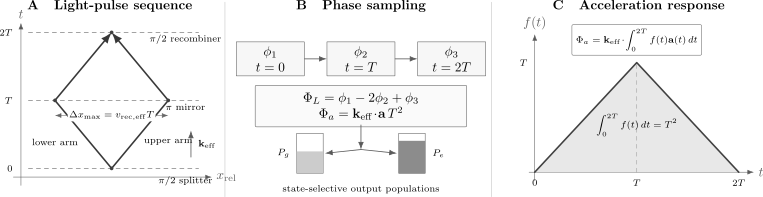
The ideal light-pulse Mach–Zehnder sequence. The atom–light phases enter as $\phi_1-2\phi_2+\phi_3$. A time-dependent acceleration is weighted by the triangular response $f(t)$; its area is $T^2$, which gives $\Phi_a=\mathbf k_{\mathrm{eff}}\mathbin{\cdot}\mathbf aT^2$ for constant relative acceleration.

Output probability

When pulse areas are ideal and unwanted ports are negligible, the two alternatives reaching one output add coherently. One output has

$$P_e = \frac12 \left[ 1+C\cos\Phi \right],$$

and the complementary output has $P_g=1-P_e$ if there is no loss or leakage. The contrast $C$ includes wave-packet overlap, ensemble averaging, pulse errors, decoherence, and detection normalization.

Laser-phase finite difference

For ideal instantaneous pulses, the imprinted phase has the structure

$$\Phi_{\mathrm{laser}} = \phi_1-2\phi_2+\phi_3,$$

where $\phi_j$ is the effective atom–light phase evaluated at the relevant interaction event. The factor $-2$ occurs because the middle mirror pulse acts once on each arm with opposite transition direction.

If the phase fronts are planar and the effective optical phase is sampled along a reference trajectory $\mathbf r(t)$,

$$\begin{aligned} \Phi_{\mathrm{laser}} \supset{}& \mathbf k_{\mathrm{eff}} \mathbin{\cdot} \big[ \mathbf r(0) -2\mathbf r(T) +\mathbf r(2T) \big]. \end{aligned}$$

For

$$\mathbf r(t) = \mathbf r_0 + \mathbf v_0t + \frac12\mathbf a t^2,$$

the position and velocity terms cancel:

$$\mathbf r(0) -2\mathbf r(T) +\mathbf r(2T) = \mathbf aT^2.$$

After the complete propagation and separation ledger is included, the closed uniform-acceleration result is

$$\Phi_a = \mathbf k_{\mathrm{eff}} \mathbin{\cdot} \mathbf aT^2.$$

Frequency chirp

A falling atom acquires a changing Doppler shift. The Raman frequency difference is commonly chirped so the pulses remain resonant. Let the synthesized phase contain

$$\varphi(t) = \varphi_0 + \omega_0t + \frac12\alpha t^2.$$

Then the quadratic phase contributes

$$-\alpha T^2$$

to the three-pulse finite difference. The leading phase becomes

$$\Phi = \left( \mathbf k_{\mathrm{eff}} \mathbin{\cdot} \mathbf a - \alpha \right) T^2 + \Phi_{\mathrm{sys}}.$$

Here $\alpha$ has angular-frequency chirp units, $\mathrm{rad\,s^{-2}}$. Scanning $\alpha$ finds the chirp that follows the atomic Doppler shift. The measurement is a comparison between atomic free fall and the laser phase fronts.

Worked rubidium scale audit

For counterpropagating light near

$$\lambda = 780\ \mathrm{nm},$$

take

$$k_{\mathrm{eff}} \simeq \frac{4\pi}{\lambda} = 1.611\times10^7\ \mathrm{m^{-1}}.$$

For $^{87}\mathrm{Rb}$ with

$$m = 1.443\times10^{-25}\ \mathrm{kg},$$

the effective recoil velocity is

$$v_{\mathrm{rec,eff}} = \frac{\hbar k_{\mathrm{eff}}}{m} = 1.177\times10^{-2}\ \mathrm{m\,s^{-1}}.$$

At $T=0.100\ \mathrm s$, the maximum relative arm separation in the ideal sequence is approximately

$$\Delta x_{\max} = v_{\mathrm{rec,eff}}T = 1.18\ \mathrm{mm}.$$

The raw phase from standard gravity is large:

$$\begin{aligned} \Phi_g &= k_{\mathrm{eff}}gT^2 \\ &\simeq 1.58\times10^6\ \mathrm{rad}. \end{aligned}$$

The corresponding resonance-following chirp is

$$\frac{\alpha}{2\pi} = \frac{k_{\mathrm{eff}}g}{2\pi} \simeq 25.1\ \mathrm{MHz\,s^{-1}}.$$

Experiments do not usually count $1.58$ million radians from zero. They chirp near the expected value and estimate the residual phase, while tracking the integer-fringe and sign conventions.

Why no mass appears

The acceleration scale factor $k_{\mathrm{eff}}T^2$ contains no explicit atomic mass. The momentum kick is $\hbar k_{\mathrm{eff}}$, so the arm velocity separation is inversely proportional to mass, while the center-of-mass action is proportional to mass. These factors cancel in the ideal uniform-acceleration phase.

Mass still matters through recoil frequency, spatial separation, source expansion, diffraction resonance, interaction effects, and response to gradients. “Mass independent” applies to the leading scale factor, not to the complete apparatus.

Avoiding a phase-story trap

It is possible to rearrange the total phase among propagation, laser, and separation terms by changing coordinates or bookkeeping. Assigning the observed phase to only a gravitational potential term, only a proper-time term, or an enormous atomic “Compton clock” phase can be misleading unless the complete gauge- and frame-consistent interferometer is shown.

The invariant object is the measured phase difference predicted by the complete atom-plus-laser model.

Acceleration Response

Time-dependent acceleration

For ideal instantaneous pulses, define

$$f(t) = \begin{cases} t, & 0<t<T, \\ 2T-t, & T<t<2T, \\ 0, & \text{otherwise}. \end{cases}$$

The acceleration phase is

$$\Phi_a = \mathbf k_{\mathrm{eff}} \mathbin{\cdot} \int_0^{2T} f(t)\mathbf a(t)\,dt.$$

For constant acceleration,

$$\int_0^{2T} f(t)\,dt = T^2,$$

recovering $\Phi_a=\mathbf k_{\mathrm{eff}}\cdot\mathbf aT^2$.

The triangular weight shows that the interferometer does not measure instantaneous acceleration at one time. It measures a time-weighted combination over the complete sequence.

Mirror vibration

In a retroreflected geometry, displacement $z_m(t)$ of the reference mirror changes the effective laser phase. For ideal pulses,

$$\Phi_{\mathrm{vib}} \simeq k_{\mathrm{eff}} \left[ z_m(0) -2z_m(T) +z_m(2T) \right]$$

under a declared sign convention. The same vibration can be written as a weighted mirror acceleration.

Because $k_{\mathrm{eff}}$ is large, submicrometer mirror motion can sweep many fringes. Isolation, a classical accelerometer, feed-forward, correlation analysis, or common-mode differential interferometers are often essential.

Laser phase noise

A laser phase perturbation sampled by the pulses contributes

$$\delta\Phi_L = \delta\phi_L(0) -2\delta\phi_L(T) +\delta\phi_L(2T)$$

in the instantaneous limit. Finite pulses replace point samples by a sensitivity function. Oscillator phase noise, optical path noise, and phase lock noise must be filtered through that transfer function, not summarized only by an integrated linewidth.

Scale-factor calibration

The leading acceleration scale factor is

$$K_a = k_{\mathrm{eff}}T^2.$$

Its uncertainty can include:

• optical frequency and beam-angle uncertainty in $k_{\mathrm{eff}}$;
• pulse-timing calibration;
• finite-pulse corrections;
• wavefront curvature sampled by an expanding ensemble;
• gravity-gradient coupling to initial position and velocity;
• Coriolis acceleration from transverse velocity;
• chirp nonlinearity; and
• differences between the phase reference point and the reported sensor location.

The formula is simple enough that neglected geometry often dominates its uncertainty.

Rotation and the Matter-Wave Sagnac Phase

Coriolis form

In a frame rotating with angular velocity $\boldsymbol\Omega$, an atom with velocity $\mathbf v$ experiences Coriolis acceleration

$$\mathbf a_C = -2 \boldsymbol\Omega \mathbin{\times} \mathbf v.$$

Inserted into the acceleration scale factor, the leading rotation phase is

$$\begin{aligned} \Phi_\Omega &= -2T^2 \mathbf k_{\mathrm{eff}} \mathbin{\cdot} \left( \boldsymbol\Omega \mathbin{\times} \mathbf v \right) \\ &= 2T^2 \mathbf k_{\mathrm{eff}} \mathbin{\cdot} \left( \mathbf v \mathbin{\times} \boldsymbol\Omega \right). \end{aligned}$$

The velocity here is relative to the rotating apparatus and must be tied to the chosen trajectory and pulse geometry.

Enclosed-area form

For a matter-wave interferometer enclosing oriented area $\mathbf A$, the nonrelativistic Sagnac phase can be written

$$\Phi_\Omega = \frac{2m}{\hbar} \boldsymbol\Omega \mathbin{\cdot} \mathbf A.$$

In a light-pulse geometry,

$$\mathbf A \sim \frac{\hbar\mathbf k_{\mathrm{eff}}}{m} \mathbin{\times} \mathbf v\,T^2,$$

which reproduces the Coriolis form up to orientation conventions.

Earth-rotation audit

For maximum geometric projection, take

$$k_{\mathrm{eff}} = 1.611\times10^7\ \mathrm{m^{-1}}, \quad v = 0.50\ \mathrm{m\,s^{-1}}, \quad T = 0.100\ \mathrm s,$$

and

$$\Omega_\oplus = 7.292\times10^{-5}\ \mathrm{rad\,s^{-1}}.$$

Then

$$\begin{aligned} |\Phi_\Omega| &\simeq 2k_{\mathrm{eff}}v\Omega_\oplus T^2 \\ &= 11.7\ \mathrm{rad}. \end{aligned}$$

Earth rotation is therefore not automatically a tiny correction. It can be the signal in a gyroscope or a bias in a vertical accelerometer. Transverse velocity, beam direction, latitude, and mirror orientation must be measured.

Gravimetry, Gradiometry, and Inertial Sensing

Absolute gravimetry

A vertical interferometer compares atomic free fall with an optical phase reference tied to an instrument structure. The chirp rate that nulls the phase estimates the projection of gravitational acceleration along $\mathbf k_{\mathrm{eff}}$ after corrections:

$$\widehat g \simeq \frac{\widehat\alpha}{k_{\mathrm{eff}}} - \frac{\widehat\Phi_{\mathrm{sys}}}{ k_{\mathrm{eff}}T^2 }.$$

The reported value must specify sensor height, tides, atmospheric loading, polar motion, local mass distribution, vertical gravity gradient, and the instrument’s effective measurement height when those effects matter.

Differential gradiometry

Operate two interferometers at positions separated by baseline $\mathbf L$, interrogated by common laser pulses. Their phase difference is

$$\Delta\Phi \simeq \mathbf k_{\mathrm{eff}} \mathbin{\cdot} \left( \mathbf a_2-\mathbf a_1 \right) T^2.$$

For a slowly varying field,

$$\mathbf a_2-\mathbf a_1 \simeq \Gamma\mathbf L,$$

where $\Gamma$ is the gravity-gradient tensor. Common laser and mirror noise can cancel strongly, but unequal scale factors, timing, Rabi frequencies, wavefront sampling, and atom trajectories limit rejection.

Accelerometers and gyroscopes

An accelerometer maximizes $\mathbf k_{\mathrm{eff}}\cdot\mathbf a$. A gyroscope arranges nonzero transverse velocity or enclosed area so that $\boldsymbol\Omega\cdot\mathbf A$ is measurable. Multi-axis instruments use several beam directions, atomic trajectories, or simultaneous interferometers.

The same phase can contain both acceleration and rotation. Geometry, modulation, reversal, and auxiliary sensors are needed to separate them.

Other applications

Atom interferometers also support:

• measurements of recoil and $h/m$;
• determinations of the fine-structure constant when combined with other constants;
• measurements of the Newtonian gravitational constant with source masses;
• tests of differential free fall;
• searches for weak or oscillatory forces;
• measurements of polarizability and electromagnetic phases; and
• long-baseline concepts for gravitational and dark-sector signals.

These applications use different observables and systematic controls. Listing them under one platform does not imply one universal sensitivity or one settled interpretation.

Wave-Packet Closure and Contrast

Closure in phase space

At recombination, corresponding wave packets should overlap in position, momentum, internal state, and all unobserved degrees of freedom. Let the residual displacement and momentum mismatch be

$$\Delta\mathbf x, \qquad \Delta\mathbf p.$$

For one one-dimensional minimum-uncertainty Gaussian of rms width $\sigma_x$, the overlap magnitude is

$$\left| \langle\psi_1|\psi_2\rangle \right| = \exp \left[ - \frac{\Delta x^2}{8\sigma_x^2} - \frac{\sigma_x^2\Delta p^2}{2\hbar^2} \right].$$

An open interferometer can therefore lose contrast even under perfectly unitary evolution. The missing visibility reflects unresolved output modes, not necessarily environmental decoherence.

Contrast is an ensemble observable

Measured contrast can be reduced by:

• incomplete pulse transfer;
• Doppler detuning across the velocity distribution;
• spatial Rabi-frequency variation;
• wavefront curvature and aberration;
• residual position or momentum mismatch;
• differential magnetic and optical phases;
• spontaneous scattering;
• collisions and mean-field evolution;
• parasitic diffraction paths;
• atom loss and background counts;
• shot-to-shot phase noise; and
• averaging over a phase that varies across the cloud.

A low contrast is not a diagnosis. One must vary controlled parameters and compare against a model that predicts both phase and contrast.

Which-path information

If an environment or uncontrolled internal degree of freedom ends in states $|E_u\rangle$ and $|E_\ell\rangle$ correlated with the two arms, the interference term is multiplied by

$$\langle E_\ell|E_u\rangle.$$

Spontaneous emission is especially destructive because the emitted photon can carry path, time, momentum, and internal-state information. Large one-photon detuning reduces excited-state population, but higher laser power may be required to preserve the two-photon Rabi rate.

Gravity gradients and open geometry

In a gravity gradient, trajectories do not close exactly under the pulse timing designed for uniform acceleration. Initial position and velocity can couple into the phase, and residual phase-space displacement can reduce contrast. Frequency shifts or modified mirror-pulse momentum transfer can help close the geometry, but the correction becomes part of the calibrated scale factor.

Detection and Phase Estimation

State-selective detection

Raman interferometers often detect the populations $N_g$ and $N_e$ by state-selective fluorescence, absorption imaging, or sequential shelving and repumping. A normalized output is

$$P_e = \frac{N_e}{ N_g+N_e },$$

after background, efficiency, and loss corrections justified by the detection model.

Normalization suppresses common atom-number fluctuations only if both state channels are linear and their relative calibration is stable.

Midfringe operation

The maximum probability slope occurs near quadrature:

$$\Phi+\phi_{\mathrm{off}} \simeq \frac{\pi}{2} \pmod{\pi}.$$

A controlled phase step on the last pulse can lock the interferometer near this point. If vibration noise spans many fringes, a nonlinear estimator can correlate atomic populations with an auxiliary accelerometer or with a second interferometer rather than linearizing one shot at a time.

Projection-noise baseline

For $N$ independent detected atoms and contrast $C$, the midfringe phase uncertainty has the approximate single-shot scale

$$\delta\Phi_{\mathrm{PN}} \simeq \frac{1}{ C\sqrt N }.$$

The corresponding acceleration uncertainty is

$$\delta a_{\mathrm{PN}} \simeq \frac{1}{ C\sqrt N\, k_{\mathrm{eff}}T^2 }.$$

For

$$N=10^6, \qquad C=0.50, \qquad T=0.100\ \mathrm s,$$

with the rubidium scale above,

$$\delta a_{\mathrm{PN}} \simeq 1.24\times10^{-8}\ \mathrm{m\,s^{-2}}$$

per shot. Detection noise, vibration, dead time, contrast fluctuations, wavefront effects, and drift commonly lie above this ideal baseline.

Sensitivity versus accuracy

Sensitivity describes statistical response or noise, often per shot or per square-root bandwidth. Accuracy concerns agreement with the defined measurand after systematic corrections. A highly sensitive interferometer can be inaccurate, and an accurate instrument can average slowly.

State the averaging time, cycle rate, bandwidth, estimator, rejection rules, and uncertainty model whenever a sensitivity or accuracy is quoted.

Platform Architectures

Atomic beams

Thermal or laser-cooled beams provide continuous flux and naturally enclose area for rotation sensing. Their broad velocity distribution requires velocity selection or geometry-aware averaging.

Drop and fountain interferometers

Cold clouds can be dropped or launched through vertically separated pulses. Longer $T$ increases the acceleration scale factor as $T^2$ but requires more apparatus height, larger beams, longer coherence, and better vibration control.

Guided and trapped interferometers

Magnetic, optical, or atom-chip guides can extend interaction time in a compact region. Confinement introduces trap roughness, interactions, anharmonicity, path-dependent potentials, and more demanding closure.

Condensate and delta-kick sources

Bose–Einstein condensates and delta-kick collimation can provide narrow momentum distributions and slow expansion. Interactions can add density-dependent phase and lensing. A narrower source is not automatically more accurate unless interaction and wavefront systematics are controlled.

Long-baseline and space concepts

Long free-fall time and large momentum transfer increase spacetime area. They also increase demands on beam size, optical phase control, gravity gradients, Coriolis compensation, timing, wave-packet closure, and environmental modeling. Projected sensitivity should be distinguished from demonstrated integrated performance.

Noise and Systematic Ledger

Laser and optical effects

• Reference-mirror vibration: enters directly through sampled optical phase.
• Laser phase noise: filtered by pulse timing and finite-pulse sensitivity.
• Wavefront aberration: maps cloud position and velocity distributions into phase.
• Beam alignment: changes the projection of $\mathbf k_{\mathrm{eff}}$ and creates transverse coupling.
• Gouy and curvature phases: make the local wave vector differ from a plane wave.
• Differential ac Stark shift: changes the internal transition during Raman pulses.
• Diffraction phase: depends on pulse intensity, detuning, and unwanted momentum ports.
• Spontaneous scattering: causes loss, decoherence, and recoil.

Atomic effects

• initial position and velocity distributions;
• residual transverse velocity coupled to rotation;
• magnetic-field gradients and quadratic Zeeman shifts;
• mean-field and collisional phases;
• unequal populations or imperfect state preparation;
• velocity-dependent pulse area;
• background-gas collisions;
• thermal expansion and clipping; and
• species- or isotope-dependent optical response in differential tests.

Inertial and gravitational effects

• Earth rotation and platform angular motion;
• gravity gradients and curvature;
• tides and nearby moving masses;
• platform tilt;
• uncertainty in effective measurement position;
• vibration aliasing and dead time; and
• coupling among acceleration, rotation, and initial conditions.

Reversal and modulation strategies

Useful discriminators include:

• reversing $\mathbf k_{\mathrm{eff}}$;
• reversing launch velocity or enclosed area;
• alternating internal magnetic sublevels;
• varying $T$ to test $T^2$ scaling;
• changing atom number to test interaction shifts;
• changing pulse intensity and detuning;
• operating simultaneous differential interferometers; and
• inserting copropagating Raman pulses to isolate internal-state shifts.

No reversal cancels everything. A systematic survives whenever the reversal changes another experimental parameter or the effect shares the same symmetry as the signal.

Calibration and Validation Workflow

1. Characterize the source

Measure atom number, internal-state purity, cloud position, velocity, temperature or covariance matrix, expansion, and shot-to-shot correlations.

2. Characterize each pulse

Map Rabi oscillations or diffraction efficiency versus duration, intensity, detuning, and velocity. Measure spontaneous loss and parasitic momentum orders. Record the optical phase reference and beam geometry.

3. Verify closure

Image output ports when possible. Vary timing, mirror-pulse frequency, momentum direction, and initial velocity. Separate reduced contrast caused by phase-space mismatch from phase noise.

4. Calibrate the phase response

Apply known laser phase steps, mirror displacements, timing changes, or frequency chirps. Verify sign, scale, linear range, and the $T^2$ dependence in the regime where the ideal model is claimed.

5. Build the detection model

Measure backgrounds, state cross-talk, atom-number linearity, saturation, loss, and assignment uncertainty. Preserve raw populations alongside normalized outputs.

6. Map systematics

Vary beam alignment, transverse velocity, magnetic field, intensity, detuning, cloud size, atom number, and apparatus orientation. Fit a physically motivated model and propagate calibration covariance.

7. Validate the integrated observable

Compare with an independent accelerometer, gravimeter, rotation reference, known source mass, or injected phase. Blind offsets and configuration reversals help distinguish analysis choices from physical response.

Minimal reproducibility package

A mature report gives:

• pulse timings and envelopes;
• optical frequencies, detunings, polarizations, and beam geometry;
• the definition and sign of $\mathbf k_{\mathrm{eff}}$;
• source distributions and internal states;
• detection and normalization equations;
• the fitted fringe or likelihood model;
• raw and corrected phase values;
• scale-factor and systematic budgets;
• calibration cadence and drift treatment; and
• data cuts and uncertainty propagation.

Common Mistakes

“The atom follows both classical paths”

The alternatives are components of one quantum state. Classical trajectories are stationary-phase tools for computing their centers and phases, not evidence that a localized classical atom secretly chose both routes.

“The first pulse splits the atom into two half-atoms”

It creates a coherent superposition of momentum and, for Raman pulses, internal-state alternatives. Detection still returns whole atoms.

“The phase is only the potential-energy integral”

Laser phases and separation terms are essential. Individual phase components can change under a frame or gauge choice while the total remains observable.

“The gravity phase proves atoms are Compton clocks”

The measured phase belongs to the complete atom–light interferometer. Rewriting one contribution using $mc^2/\hbar$ does not by itself establish an independently oscillating clock at that frequency.

“Colder always means more accurate”

Lower expansion can reduce wavefront averaging, but condensate interactions, source correlations, and selection effects can introduce other biases.

“Contrast loss proves environmental decoherence”

Pulse inhomogeneity, open phase-space geometry, unresolved momentum ports, and shot-to-shot phase noise can reduce ensemble contrast without irreversible environmental which-path records.

“The scale factor is exactly k effective T squared”

That is the instantaneous-pulse, uniform-acceleration leading term. Finite pulses, gradients, rotation, wavefronts, timing, and geometry modify the response.

“Reversing k removes all systematics”

It rejects effects with the opposite reversal parity only when both configurations are otherwise identical.

“A beautiful fringe is a calibrated sensor”

A fringe establishes coherent phase response. A sensor claim additionally needs a transfer function, estimator, noise spectrum, systematic budget, traceability, and stability record.

Exercises

1. Raman recoil scales

For counterpropagating Raman beams at $\lambda=780\ \mathrm{nm}$ acting on $^{87}\mathrm{Rb}$ with mass

$$m=1.443\times10^{-25}\ \mathrm{kg},$$

calculate:

1. $k_{\mathrm{eff}}\simeq4\pi/\lambda$;
2. the effective recoil velocity $v_{\mathrm{rec,eff}}=\hbar k_{\mathrm{eff}}/m$; and
3. the effective recoil frequency $f_{\mathrm{rec,eff}}=\hbar^2k_{\mathrm{eff}}^2/(2mh)$.

Solution

The effective wave number is

$$\begin{aligned} k_{\mathrm{eff}} &= \frac{4\pi}{780\times10^{-9}\ \mathrm m} \\ &= 1.611\times10^7\ \mathrm{m^{-1}}. \end{aligned}$$

The recoil velocity is

$$\begin{aligned} v_{\mathrm{rec,eff}} &= \frac{ (1.0546\times10^{-34}) (1.611\times10^7) }{ 1.443\times10^{-25} } \\ &= 1.18\times10^{-2}\ \mathrm{m\,s^{-1}}. \end{aligned}$$

The kinetic recoil frequency is

$$\begin{aligned} f_{\mathrm{rec,eff}} &= \frac{ \hbar^2k_{\mathrm{eff}}^2 }{ 2mh } \\ &\simeq 1.51\times10^4\ \mathrm{Hz}. \end{aligned}$$

This is four times the single-photon recoil frequency because $k_{\mathrm{eff}}\simeq2k$ and recoil energy scales as wave number squared.

2. Separation and gravity phase

Use the recoil velocity from Exercise 1 and $T=0.100\ \mathrm s$.

1. Find the maximum arm separation.
2. Find the ideal phase from $g=9.80665\ \mathrm{m\,s^{-2}}$.
3. Explain why the large phase does not require measuring from zero phase.

Solution

The maximum separation occurs near the mirror pulse:

$$\Delta x_{\max} = v_{\mathrm{rec,eff}}T = (1.177\times10^{-2})(0.100) = 1.18\ \mathrm{mm}.$$

The phase is

$$\begin{aligned} \Phi_g &= k_{\mathrm{eff}}gT^2 \\ &= (1.611\times10^7) (9.80665) (0.100)^2 \\ &= 1.58\times10^6\ \mathrm{rad}. \end{aligned}$$

The Raman frequency difference is chirped near the expected Doppler rate, which subtracts nearly all of this phase. The experiment estimates a residual phase or the chirp value that nulls it. Configuration reversals and prior knowledge keep track of fringe order.

3. Chirp-rate null

For the geometry in Exercise 2, calculate the frequency chirp $\alpha/(2\pi)$ that nulls the leading gravity phase. If the applied chirp is larger by $100\ \mathrm{Hz\,s^{-1}}$, what residual phase appears at $T=0.100\ \mathrm s$?

Solution

The null condition is

$$\alpha = k_{\mathrm{eff}}g.$$

In ordinary-frequency chirp units,

$$\begin{aligned} \frac{\alpha}{2\pi} &= \frac{k_{\mathrm{eff}}g}{2\pi} \\ &= 25.1\ \mathrm{MHz\,s^{-1}}. \end{aligned}$$

An excess ordinary-frequency chirp of $100\ \mathrm{Hz\,s^{-1}}$ corresponds to angular chirp error

$$\delta\alpha = 2\pi(100)\ \mathrm{rad\,s^{-2}}.$$

The residual phase is

$$\delta\Phi = -\delta\alpha T^2 = -2\pi(100)(0.100)^2 = -2\pi\ \mathrm{rad}.$$

That is one complete fringe. The sign follows the chirp convention used in the page.

4. Use the triangular response

An extra constant acceleration $\delta a$ acts only during the first half of the sequence, $0<t<T$, and vanishes for $T<t<2T$. Find its phase contribution. Compare it with the phase from the same acceleration acting throughout the full sequence.

Solution

During the first interval, $f(t)=t$. Therefore

$$\begin{aligned} \delta\Phi_{\mathrm{first}} &= k_{\mathrm{eff}} \int_0^T t\,\delta a\,dt \\ &= \frac12 k_{\mathrm{eff}}\delta aT^2. \end{aligned}$$

If the same acceleration acts during the whole sequence,

$$\delta\Phi_{\mathrm{full}} = k_{\mathrm{eff}}\delta aT^2.$$

The first interval contributes half because the triangular response has equal area before and after the mirror pulse.

5. Earth-rotation phase

Assume the vectors are oriented for maximum projection and use

$$k_{\mathrm{eff}} = 1.611\times10^7\ \mathrm{m^{-1}}, \quad v=0.50\ \mathrm{m\,s^{-1}}, \quad T=0.100\ \mathrm s,$$

with

$$\Omega_\oplus = 7.292\times10^{-5}\ \mathrm{rad\,s^{-1}}.$$

Estimate the Coriolis rotation phase. What reversals help distinguish it from linear acceleration?

Solution

For maximum projection,

$$\begin{aligned} |\Phi_\Omega| &= 2k_{\mathrm{eff}}v\Omega_\oplus T^2 \\ &= 2 (1.611\times10^7) (0.50) (7.292\times10^{-5}) (0.100)^2 \\ &= 11.7\ \mathrm{rad}. \end{aligned}$$

Reversing transverse velocity reverses the rotation phase but not the leading acceleration phase. Reversing $\mathbf k_{\mathrm{eff}}$ reverses both. Combining momentum and velocity reversals, or comparing oppositely directed atomic trajectories, separates their reversal parities.

6. Projection-noise acceleration scale

An interferometer detects $N=10^6$ independent atoms per shot with contrast $C=0.50$. Use $T=0.100\ \mathrm s$ and $k_{\mathrm{eff}}=1.611\times10^7\ \mathrm{m^{-1}}$.

1. Estimate the midfringe phase uncertainty.
2. Convert it to acceleration uncertainty.
3. Name three effects omitted from this baseline.

Solution

The phase scale is

$$\delta\Phi_{\mathrm{PN}} = \frac{1}{C\sqrt N} = \frac{1}{(0.50)(1000)} = 2.0\times10^{-3}\ \mathrm{rad}.$$

The acceleration scale factor is

$$k_{\mathrm{eff}}T^2 = 1.611\times10^5\ \mathrm{s^2\,m^{-1}},$$

so

$$\begin{aligned} \delta a_{\mathrm{PN}} &= \frac{\delta\Phi_{\mathrm{PN}}}{ k_{\mathrm{eff}}T^2 } \\ &= 1.24\times10^{-8}\ \mathrm{m\,s^{-2}} \end{aligned}$$

per shot. Omitted effects include detection noise, vibration, laser phase noise, wavefront aberration, finite-pulse corrections, atom-number and contrast fluctuations, dead time, rotation uncertainty, and systematic drift.

7. Wave-packet overlap

Two one-dimensional Gaussian output packets have common rms width $\sigma_x=50\ \mu\mathrm m$, residual displacement $\Delta x=20\ \mu\mathrm m$, and residual velocity mismatch $\Delta v=5.0\ \mu\mathrm{m\,s^{-1}}$ for $^{87}\mathrm{Rb}$. Estimate their overlap magnitude using

$$\left| \langle\psi_1|\psi_2\rangle \right| = \exp \left[ - \frac{\Delta x^2}{8\sigma_x^2} - \frac{\sigma_x^2m^2\Delta v^2}{2\hbar^2} \right].$$

Solution

The position-mismatch exponent is

$$\frac{\Delta x^2}{8\sigma_x^2} = \frac{(20)^2}{8(50)^2} = 0.020.$$

For

$$m=1.443\times10^{-25}\ \mathrm{kg},$$

the momentum-mismatch exponent is

$$\frac{\sigma_x^2m^2\Delta v^2}{2\hbar^2} \simeq 0.0585.$$

Thus

$$\left| \langle\psi_1|\psi_2\rangle \right| = \exp[-(0.020+0.0585)] \simeq 0.924.$$

Even a unitary interferometer can lose about $7.6\%$ of ideal amplitude visibility from this unresolved phase-space mismatch. An ensemble may lose more through averaging over packet parameters.

8. Validate an accelerometer claim

Design a validation program for a new vertical light-pulse atom accelerometer. Your answer must include:

1. source characterization;
2. pulse and momentum-transfer calibration;
3. phase-scale calibration;
4. vibration treatment;
5. rotation and wavefront tests;
6. state-detection validation;
7. at least two reversals; and
8. a criterion that would falsify the claimed simple scale factor.

Solution

One defensible program is:

1. Measure cloud position, velocity, covariance, internal-state purity, atom number, and expansion on every configuration.
2. Map Raman Rabi oscillations and velocity-sensitive spectra to determine pulse area, Doppler acceptance, recoil direction, parasitic transfer, and spontaneous loss.
3. Inject known phase steps and chirp offsets. Verify the sign and local slope of the output fringe, then repeat at several $T$ values to test $T^2$ scaling.
4. Record mirror motion with an independently calibrated accelerometer. Compare feed-forward and correlation estimates and verify residuals against the sensitivity function.
5. Vary transverse launch velocity, apparatus tilt, cloud size, and beam position to map Coriolis and wavefront couplings.
6. Calibrate fluorescence backgrounds, state cross-talk, saturation, loss, and normalized-population bias.
7. Reverse $\mathbf k_{\mathrm{eff}}$ and transverse velocity. Also vary Raman intensity and magnetic sublevel to identify even and odd systematic phases.
8. Compare against an independent acceleration reference or a controlled mirror displacement.

The simple scale-factor model is falsified at the claimed uncertainty if the fitted response does not scale as $k_{\mathrm{eff}}T^2$ after measured finite-pulse corrections, or if configuration reversals reveal an unmodeled phase that is degenerate with acceleration.

References

1. C. J. Bordé, “Atomic interferometry with internal state labelling,” Physics Letters A 140, 10–12 (1989), doi:10.1016/0375-9601(89)90537-9.
2. O. Carnal and J. Mlynek, “Young’s double-slit experiment with atoms: A simple atom interferometer,” Physical Review Letters 66, 2689–2692 (1991), doi:10.1103/PhysRevLett.66.2689.
3. D. W. Keith, C. R. Ekstrom, Q. A. Turchette, and D. E. Pritchard, “An interferometer for atoms,” Physical Review Letters 66, 2693–2696 (1991), doi:10.1103/PhysRevLett.66.2693.
4. M. Kasevich and S. Chu, “Atomic interferometry using stimulated Raman transitions,” Physical Review Letters 67, 181–184 (1991), doi:10.1103/PhysRevLett.67.181.
5. M. Kasevich and S. Chu, “Measurement of the gravitational acceleration of an atom with a light-pulse atom interferometer,” Applied Physics B 54, 321–332 (1992), doi:10.1007/BF00325375.
6. P. Storey and C. Cohen-Tannoudji, “The Feynman path integral approach to atomic interferometry: A tutorial,” Journal de Physique II 4, 1999–2027 (1994), doi:10.1051/jp2:1994103.
7. T. L. Gustavson, P. Bouyer, and M. A. Kasevich, “Precision rotation measurements with an atom interferometer gyroscope,” Physical Review Letters 78, 2046–2049 (1997), doi:10.1103/PhysRevLett.78.2046.
8. A. Peters, K. Y. Chung, and S. Chu, “Measurement of gravitational acceleration by dropping atoms,” Nature 400, 849–852 (1999), doi:10.1038/23655.
9. J. M. McGuirk, G. T. Foster, J. B. Fixler, M. J. Snadden, and M. A. Kasevich, “Sensitive absolute-gravity gradiometry using atom interferometry,” Physical Review A 65, 033608 (2002), doi:10.1103/PhysRevA.65.033608.
10. P. R. Berman, editor, Atom Interferometry, Academic Press (1997).
11. A. D. Cronin, J. Schmiedmayer, and D. E. Pritchard, “Optics and interferometry with atoms and molecules,” Reviews of Modern Physics 81, 1051–1129 (2009), doi:10.1103/RevModPhys.81.1051.
12. P. Cheinet, B. Canuel, F. Pereira Dos Santos, A. Gauguet, F. Yver-Leduc, and A. Landragin, “Measurement of the sensitivity function in a time-domain atomic interferometer,” IEEE Transactions on Instrumentation and Measurement 57, 1141–1148 (2008), doi:10.1109/TIM.2007.915148.
13. H. Müller, S.-W. Chiow, Q. Long, S. Herrmann, and S. Chu, “Atom interferometry with up to 24-photon-momentum-transfer beam splitters,” Physical Review Letters 100, 180405 (2008), doi:10.1103/PhysRevLett.100.180405.
14. A. Louchet-Chauvet et al., “The influence of transverse motion within an atomic gravimeter,” New Journal of Physics 13, 065025 (2011), doi:10.1088/1367-2630/13/6/065025.
15. R. Geiger et al., “Detecting inertial effects with airborne matter-wave interferometry,” Nature Communications 2, 474 (2011), doi:10.1038/ncomms1479.
16. B. Barrett et al., “Mobile and remote inertial sensing with atom interferometers,” Reports on Progress in Physics 77, 126401 (2014), doi:10.1088/0034-4885/77/12/126401.
17. G. Rosi, F. Sorrentino, L. Cacciapuoti, M. Prevedelli, and G. M. Tino, “Precision measurement of the Newtonian gravitational constant using cold atoms,” Nature 510, 518–521 (2014), doi:10.1038/nature13433.
18. A. Roura, “Circumventing Heisenberg’s uncertainty principle in atom interferometry tests of the equivalence principle,” Physical Review Letters 118, 160401 (2017), doi:10.1103/PhysRevLett.118.160401.
19. R. H. Parker, C. Yu, W. Zhong, B. Estey, and H. Müller, “Measurement of the fine-structure constant as a test of the Standard Model,” Science 360, 191–195 (2018), doi:10.1126/science.aap7706.
20. P. Asenbaum, C. Overstreet, M. Kim, J. Curti, and M. A. Kasevich, “Atom-interferometric test of the equivalence principle at the $10^{-12}$ level,” Physical Review Letters 125, 191101 (2020), doi:10.1103/PhysRevLett.125.191101.

Cross-Links

• Interference With Matter gives the historical matter-wave context.
• Interferometry gives the cross-platform experimental logic.
• Ramsey Interferometry develops internal-state separated-pulse interference and clock readout.
• Optical Interferometers develops optical Mach–Zehnder transformations and phase-estimation statistics.
• Beam Splitters develops the optical two-port unitary and phase conventions.
• Laser Cooling owns source cooling and recoil budgets.
• Ultracold Atoms owns ultracold source preparation and diagnostics.
• Optical Lattices develops band motion and Bloch acceleration used in large-momentum transfer.
• Precision Measurement and Metrology supplies the measurand, stability, covariance, reversal, and independent-validation framework used to turn an interferometer into a sensor.
• Quantum Sensing gives the general estimator and decoherence-limited sensing framework.
• Decoherence Timescales distinguishes visibility decay from population and phase-relaxation times.