Doppler Cooling

Doppler cooling uses the velocity dependence of near-resonant photon scattering to create a force that opposes motion. In optical molasses, counterpropagating red-detuned beams make an atom preferentially absorb from the beam traveling against its velocity. The average momentum drifts toward zero while random absorption and spontaneous-emission recoils diffuse it away from zero.

The standard Doppler temperature is therefore not obtained from the mean force alone. It follows from a declared friction–diffusion model:

$$F \simeq -\alpha v, \qquad k_{\mathrm B}T = \frac{D_p}{\alpha}.$$

For weak saturation, a broad closed two-level transition, three orthogonal beam pairs, and isotropic spontaneous emission, minimizing this ratio gives

$$k_{\mathrm B}T_D = \frac{\hbar\Gamma}{2}.$$

This result is a benchmark of a specific model, not a universal floor. Multilevel polarization gradients, dark states, narrow transitions, quantized motion, and technical noise all change the mechanism or its limit.

Canonical Scope

This page owns the textbook Doppler-cooling derivation:

1. red detuning and the Doppler sign;
2. velocity-dependent absorption from counterpropagating beams;
3. one-dimensional and three-dimensional optical molasses;
4. the low-velocity friction coefficient;
5. the recoil-diffusion ledger;
6. the Doppler temperature and its optimal detuning;
7. capture, damping time, saturation, and beam balance;
8. the assumptions that fail for real atoms, ions, and molecules.

Laser Cooling owns the broader cooling taxonomy, thermometry, phase-space metrics, staged cooling architecture, and comparison with dark-state, Raman, sideband, cavity, and molecular methods. Radiation Pressure owns the general scattering-force derivation, photon momentum ledger, saturation, and force-noise conventions. Optical Bloch Equations owns the internal driven steady state.

Sub-Doppler Cooling treats polarization gradients, Sisyphus cycles, dark states, and Raman sidebands. This page uses an ideal two-level atom precisely so that the Doppler result and its failure boundary remain visible.

Assumptions

Begin with a particle of mass $m$ and a closed transition $|g\rangle\leftrightarrow|e\rangle$ of angular frequency $\omega_0$. The excited-state population decays at rate $\Gamma$. Assume:

• nonrelativistic center-of-mass motion;
• one ground state and one excited state;
• no branching or dark states;
• plane-wave beams;
• weak saturation unless stated otherwise;
• internal steady state at each velocity;
• independent beam scattering rates;
• negligible interbeam coherence and standing-wave structure;
• a dilute gas of independent particles;
• free-space spontaneous emission;
• a velocity distribution narrow enough for the low-velocity expansion when a temperature is inferred.

These assumptions are intentionally restrictive. They define the result.

Detuning and Doppler Conventions

Use atom-minus-laser detuning:

$$\Delta = \omega_0-\omega_L.$$

Red detuning means

$$\omega_L<\omega_0, \qquad \Delta>0.$$

For a beam with wave vector $\mathbf k$, the laser frequency in the particle’s rest frame is, to first order in $v/c$,

$$\omega_L' \simeq \omega_L -\mathbf k\mathbin{\cdot}\mathbf v.$$

The rest-frame atom-minus-laser detuning is

$$\Delta_v = \omega_0-\omega_L' = \Delta+\mathbf k\mathbin{\cdot}\mathbf v.$$

This sign should be derived, not memorized. References using $\delta=\omega_L-\omega_0$ assign red detuning $\delta<0$ and write $\delta_v=\delta-\mathbf k\mathbin{\cdot}\mathbf v$.

One Traveling Beam

For a closed two-level atom, define the on-resonance saturation parameter

$$s = \frac{2|\Omega|^2}{\Gamma^2},$$

where the rotating-frame Hamiltonian has off-diagonal coefficient $\hbar\Omega/2$.

The steady scattering rate is

$$R_{\mathrm{sc}}(\Delta_v) = \frac{\Gamma}{2} \frac{ s }{ 1+s+ \left( 2\Delta_v/\Gamma \right)^2 }.$$

When the mean spontaneous recoil vanishes, the beam exerts

$$\mathbf F_{\mathrm{sc}} = \hbar\mathbf k R_{\mathrm{sc}}.$$

A single beam can slow atoms arriving from one direction. It does not create a force that vanishes at $v=0$ and changes sign with velocity. Symmetric molasses requires at least a counterpropagating pair.

Counterpropagating Beams

Take two equal beams along $\pm x$ with wave vectors $\mathbf k_\pm=\pm k\hat{\mathbf x}$. For velocity $\mathbf v=v\hat{\mathbf x}$,

$$\Delta_+(v) = \Delta+kv,$$ $$\Delta_-(v) = \Delta-kv.$$

The $+x$ beam supplies positive momentum, while the $-x$ beam supplies negative momentum.

Why red detuning damps

Let $v>0$. The counterpropagating $-x$ beam has detuning $\Delta-kv$, which is smaller than $\Delta$ and therefore closer to resonance while $kv<\Delta$. The copropagating $+x$ beam has detuning $\Delta+kv$ and is farther from resonance.

The particle scatters more photons from the $-x$ beam and receives a net negative momentum kick. For $v<0$, the roles reverse. This is a restoring force in velocity space.

Weak-saturation force

To keep the beam rates additive, take $s\ll1$ and define

$$R(\delta) = \frac{\Gamma s}{2} \frac{1}{ 1+ \left( 2\delta/\Gamma \right)^2 }.$$

The net force is

$$F(v) = \hbar k \left[ R(\Delta+kv) -R(\Delta-kv) \right].$$

Equivalently,

$$F(v) = \frac{\hbar k\Gamma s}{2} \left\{ \frac{1}{ 1+ \left[ 2(\Delta+kv)/\Gamma \right]^2 } - \frac{1}{ 1+ \left[ 2(\Delta-kv)/\Gamma \right]^2 } \right\}.$$

At $v=0$, equal beams cancel:

$$F(0)=0.$$

At large $|v|$, both beams are far from resonance and $F(v)\to0$. The force is strongest when one Doppler-shifted beam approaches resonance, around $|v|\sim\Delta/k$.

Low-Velocity Friction

Expand each rate about $v=0$:

$$R(\Delta\pm kv) \simeq R(\Delta) \pm kvR'(\Delta).$$

Then

$$F(v) \simeq 2\hbar k^2vR'(\Delta).$$

With

$$R'(\Delta) = -\frac{ 4s(\Delta/\Gamma) }{ \left[ 1+ \left( 2\Delta/\Gamma \right)^2 \right]^2 },$$

the force becomes

$$F(v) \simeq -\alpha v,$$

where

$$\alpha = 8\hbar k^2s \frac{ \Delta/\Gamma }{ \left[ 1+ \left( 2\Delta/\Gamma \right)^2 \right]^2 }.$$

For red detuning $\Delta>0$, $\alpha>0$. The mean velocity obeys

$$m\frac{d\langle v\rangle}{dt} = -\alpha\langle v\rangle,$$

so

$$\langle v(t)\rangle = \langle v(0)\rangle \exp\left( -\frac{t}{\tau_v} \right),$$

with damping time

$$\tau_v = \frac{m}{\alpha}.$$

The kinetic-energy variance relaxes twice as fast in the ideal Ornstein–Uhlenbeck model because it is quadratic in velocity.

Maximum damping is not minimum temperature

Write $d=\Delta/\Gamma$. Apart from constants,

$$\alpha(d) \propto \frac{ d }{ \left( 1+4d^2 \right)^2 }.$$

Differentiating shows that the friction coefficient is largest at

$$d = \frac{1}{2\sqrt{3}},$$

or

$$\Delta = \frac{\Gamma}{2\sqrt{3}}.$$

The Doppler temperature will instead be minimized at $\Delta=\Gamma/2$. Fastest local damping and coldest steady state are different optimization targets.

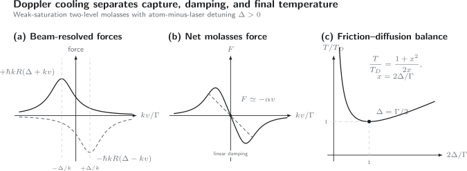
At red detuning, the two directed Lorentzian forces cancel at $v=0$ but have opposite Doppler shifts. Their difference has a negative low-velocity slope, $F\simeq-\alpha v$. Recoil diffusion prevents collapse to zero momentum. In the weak-saturation textbook model, $T/T_D=(1+x^2)/(2x)$ with $x=2\Delta/\Gamma$, and the minimum occurs at $\Delta=\Gamma/2$.

Optical Molasses

Optical molasses is a configuration of nearly balanced beams that damps velocity near zero without, by itself, providing stable position confinement.

Three-dimensional arrangement

The standard idealization uses three orthogonal counterpropagating pairs:

$$\pm k\hat{\mathbf x}, \qquad \pm k\hat{\mathbf y}, \qquad \pm k\hat{\mathbf z}.$$

If the axes are independent and equivalent,

$$\mathbf F \simeq -\alpha\mathbf v.$$

The low-velocity mechanical energy obeys

$$\frac{d}{dt} \left\langle \frac{1}{2}mv^2 \right\rangle_{\mathrm{fric}} = -\alpha \left\langle v^2\right\rangle.$$

Spontaneous recoil and random absorption add energy. Steady state is reached when this cooling power balances diffusion.

No positional restoring force

If the beams are uniform and balanced,

$$\mathbf F(\mathbf r,\mathbf 0) \simeq 0$$

throughout the overlap region. A displaced stationary atom is not pushed back toward the center. Beam edges can provide accidental spatial effects, but they are not the controlled restoring mechanism of a trap.

A magneto-optical trap adds magnetic-field-dependent detunings and polarization selection so that the scattering imbalance depends on position. Molasses and a magneto-optical trap should not be treated as synonyms.

Coherence caveat

Six beams derived from common lasers can form standing waves and polarization gradients. Treating them as independent rates requires frequency offsets, phase averaging, motion, or another reason that coherent interference is negligible for the observable.

The very interference and multilevel structure neglected by the two-level molasses model can generate sub-Doppler cooling.

Momentum Diffusion

The average spontaneous recoil may vanish, but its variance does not.

Pair scattering rate

At $v=0$, one beam scatters at rate

$$R_0 = \frac{\Gamma s}{2} \frac{1}{ 1+ \left( 2\Delta/\Gamma \right)^2 }.$$

One beam pair therefore scatters at total rate

$$R_{\mathrm{pair}} = 2R_0 = \frac{\Gamma s}{ 1+ \left( 2\Delta/\Gamma \right)^2 }.$$

Define

$$D = 1+ \left( 2\Delta/\Gamma \right)^2.$$

Then

$$R_{\mathrm{pair}} = \frac{\Gamma s}{D}.$$

Absorption contribution along one axis

At zero mean velocity, absorption from the $\pm x$ beams occurs with equal probability. Each event contributes $\pm\hbar k$ along $x$. The absorption part of the variance growth is

$$\frac{d}{dt} \operatorname{Var}(p_x) \bigg|_{\mathrm{abs}} = (\hbar k)^2 R_{\mathrm{pair}}.$$

Absorption from the $y$ and $z$ beam pairs has no $x$ projection in this plane-wave idealization.

Spontaneous-emission contribution

There are three beam pairs, so the total scattering rate is $3R_{\mathrm{pair}}$. For isotropic emission,

$$\left\langle k_{s,x}^2 \right\rangle = \frac{k^2}{3}.$$

The spontaneous-emission contribution along $x$ is therefore

$$\frac{d}{dt} \operatorname{Var}(p_x) \bigg|_{\mathrm{sp}} = \frac{(\hbar k)^2}{3} \left( 3R_{\mathrm{pair}} \right) = (\hbar k)^2 R_{\mathrm{pair}}.$$

The absorption and spontaneous parts are equal in this symmetric 3D model.

Diffusion coefficient

Using

$$\frac{d}{dt} \operatorname{Var}(p_x) = 2D_p,$$

the two contributions give

$$D_p = (\hbar k)^2 R_{\mathrm{pair}}.$$

Hence

$$D_p = \hbar^2k^2 \frac{\Gamma s}{D}.$$

This numerical result depends on the geometry and diffusion convention. Dipole emission patterns, unequal beam intensities, reduced dimensionality, and multilevel optical pumping alter it.

Deriving the Doppler Temperature

For one Cartesian component, the low-velocity Fokker–Planck equation is

$$\frac{\partial f}{\partial t} = \frac{\alpha}{m} \frac{\partial}{\partial p} \left( pf \right) + D_p \frac{\partial^2f}{\partial p^2}.$$

Its stationary Gaussian has

$$\left\langle p^2\right\rangle = \frac{mD_p}{\alpha}.$$

Identifying

$$\left\langle p^2\right\rangle = mk_{\mathrm B}T$$

gives

$$k_{\mathrm B}T = \frac{D_p}{\alpha}.$$

Substitute

$$D_p = \frac{\hbar^2k^2\Gamma s}{D},$$

and

$$\alpha = 8\hbar k^2s \frac{ \Delta/\Gamma }{ D^2 }.$$

The factors $k^2$ and $s$ cancel:

$$k_{\mathrm B}T(\Delta) = \frac{\hbar\Gamma}{8} \frac{ D }{ \Delta/\Gamma }.$$

Define

$$x = \frac{2\Delta}{\Gamma}.$$

Then

$$k_{\mathrm B}T(x) = \frac{\hbar\Gamma}{4} \frac{ 1+x^2 }{ x }.$$

Optimize the detuning

For $x>0$,

$$\frac{d}{dx} \left( \frac{1+x^2}{x} \right) = 1-\frac{1}{x^2}.$$

The minimum is at

$$x=1,$$

or

$$\Delta_{\mathrm{opt}} = \frac{\Gamma}{2}.$$

At this detuning,

$$k_{\mathrm B}T_D = \frac{\hbar\Gamma}{2}.$$

If the natural linewidth is quoted as an ordinary frequency $\gamma=\Gamma/(2\pi)$, the same result is

$$k_{\mathrm B}T_D = \frac{h\gamma}{2}.$$

Mixing $\Gamma$ in rad s$^{-1}$ with $h$ instead of $\hbar$ creates a factor-of-$2\pi$ error.

Why intensity cancels

In weak saturation, both friction and diffusion are proportional to intensity:

$$\alpha\propto s, \qquad D_p\propto s.$$

Their ratio is intensity independent. Lower intensity slows the cooling rate without changing the ideal weak-field temperature. This cancellation fails once power broadening, technical noise, finite interaction time, or other heating channels matter.

Saturation and Power Broadening

At finite intensity, the response linewidth broadens and beams share the same internal-state populations. A representative two-level expression uses an effective total saturation parameter $s_{\mathrm{tot}}$:

$$k_{\mathrm B}T \simeq \frac{\hbar\Gamma}{4} \frac{ 1+s_{\mathrm{tot}}+x^2 }{ x }.$$

Within this convention, the optimum moves to

$$x_{\mathrm{opt}} = \sqrt{1+s_{\mathrm{tot}}},$$

and

$$T_{\min} \simeq T_D \sqrt{1+s_{\mathrm{tot}}}.$$

The exact coefficient assigned to $s_{\mathrm{tot}}$ depends on whether $s$ denotes one beam, one pair, or the total field and on how cross-saturation and diffusion are modeled. The robust conclusion is that strong saturation increases capture and force but broadens the response and raises the two-level Doppler temperature.

Capture and Cooling Rate

Resonant velocity classes

The $-x$ beam is resonant when

$$\Delta-kv=0,$$

so

$$v = \frac{\Delta}{k}.$$

The $+x$ beam is resonant near $v=-\Delta/k$. At the temperature-optimal detuning, these velocities are

$$|v_{\mathrm{res}}| = \frac{\Gamma}{2k}.$$

The force remains nonzero beyond those velocities, but its magnitude falls as both beams move far off resonance. A practical capture velocity depends on:

• power-broadened linewidth;
• available beam diameter and interaction time;
• initial velocity and direction;
• maximum deceleration;
• frequency chirps or sidebands;
• gravity and magnetic fields;
• the required capture probability.

There is no universal definition of the capture velocity.

Stopping condition

For a beam of usable length $\ell$, an atom of initial speed $v_i$ requires mean deceleration

$$\bar a \gtrsim \frac{ v_i^2-v_f^2 }{ 2\ell }.$$

This must be compared with the velocity-dependent scattering acceleration, not only with the resonant ceiling

$$a_{\max} = \frac{\hbar k\Gamma}{2m}.$$

Ordinary molasses is typically a final capture and cooling stage after a slower or precooling stage has reduced the incoming velocity.

Finite cooling time

The local damping time is

$$\tau_v = \frac{m}{\alpha}.$$

Reaching the steady Doppler temperature also requires:

• enough time within the beam overlap;
• negligible loss;
• approximately stationary beam parameters;
• a distribution lying mostly in the damping region;
• no slower reheating process that dominates at late time.

An experimentally optimized cooling duration can be finite even though the ideal linear model approaches equilibrium monotonically.

Worked Example: Rubidium Optical Molasses

Take $^{87}\mathrm{Rb}$ near $\lambda=780.24\ \mathrm{nm}$ with

$$\frac{\Gamma}{2\pi} = 6.07\ \mathrm{MHz}, \qquad m = 1.443\times10^{-25}\ \mathrm{kg}.$$

The wave number is

$$k \simeq 8.05\times10^6\ \mathrm{m^{-1}}.$$

Choose weak per-beam saturation $s=0.10$ and the temperature-optimal detuning

$$\Delta = \frac{\Gamma}{2}.$$

Doppler temperature

The ideal two-level temperature is

$$T_D = \frac{\hbar\Gamma}{2k_{\mathrm B}} \simeq 146\ \mu\mathrm K.$$

The corresponding one-dimensional rms velocity is

$$\sigma_v = \sqrt{ \frac{k_{\mathrm B}T_D}{m} } \simeq 0.118\ \mathrm{m\,s^{-1}}.$$

Friction coefficient

At $\Delta/\Gamma=1/2$,

$$\alpha = \frac{ 8\hbar k^2s(1/2) }{ \left[ 1+1 \right]^2 } = s\hbar k^2.$$

Numerically,

$$\alpha \simeq 6.84\times10^{-22}\ \mathrm{kg\,s^{-1}}.$$

The local velocity damping time is

$$\tau_v = \frac{m}{\alpha} \simeq 0.211\ \mathrm{ms}.$$

This short time applies only within the low-velocity, weak-saturation, steady-state model.

Resonant velocity and linewidth scale

The counterpropagating beam is resonant near

$$v_{\mathrm{res}} = \frac{\Delta}{k} = \frac{\Gamma}{2k} \simeq 2.37\ \mathrm{m\,s^{-1}}.$$

The broader scale $\Gamma/k$ is about $4.73\ \mathrm{m\,s^{-1}}$. These velocities are far below a room-temperature atomic-beam speed, which is why a Zeeman slower, chirped slowing, or another precapture stage is needed.

Interpretation

The ideal $146\ \mu\mathrm K$ result is much warmer than the rubidium recoil temperature, about $0.18\ \mu\mathrm K$. Real alkali molasses often enters a multilevel polarization-gradient regime and can cool below the two-level Doppler value. Agreement with $T_D$ is therefore not expected automatically, even when the apparatus is working well.

Beam Imbalance

Let the two weak-saturation parameters be

$$s_+ = s(1+\epsilon), \qquad s_- = s(1-\epsilon),$$

with $|\epsilon|\ll1$. At $v=0$, the force no longer cancels. Using

$$D = 1+ \left( 2\Delta/\Gamma \right)^2,$$

the offset force is

$$F_0 \simeq \hbar k \frac{\Gamma s\epsilon}{D}.$$

Near zero velocity,

$$F(v) \simeq F_0-\alpha v.$$

The stable drift velocity is

$$v_{\mathrm d} \simeq \frac{F_0}{\alpha} = \frac{ \Gamma\epsilon D }{ 8k(\Delta/\Gamma) }.$$

At $\Delta=\Gamma/2$,

$$v_{\mathrm d} \simeq \frac{\Gamma\epsilon}{2k}.$$

Thus a small power imbalance can displace the center of the velocity distribution by a substantial fraction of its thermal width. Temperature and mean drift should be fitted separately.

Gravity and External Forces

Add a constant external force $F_{\mathrm ext}$. In the linear regime,

$$m\dot v = F_{\mathrm ext} -\alpha v.$$

The steady drift is

$$v_{\mathrm d} = \frac{F_{\mathrm ext}}{\alpha}.$$

For gravity along the cooling axis,

$$v_{\mathrm d} = \frac{mg}{\alpha}.$$

If this drift leaves the linear force range, the full nonlinear force must be solved. Narrow-line cooling is especially sensitive because optical force, linewidth, recoil, and gravity can be comparable.

Gravity does not change the basic sign of Doppler friction, but it changes the operating point and can produce spatial sag when confinement is present.

Extension to Three Dimensions

The scalar model generalizes locally to

$$F_i \simeq -\sum_j \alpha_{ij}v_j +F_{0,i},$$

with diffusion tensor

$$\frac{d}{dt} \operatorname{Cov}(p_i,p_j) \bigg|_{\mathrm{diff}} = 2D_{ij}.$$

For perfectly orthogonal, balanced, incoherent, equal-intensity beams and an isotropic two-level transition,

$$\alpha_{ij} = \alpha\delta_{ij}, \qquad D_{ij} = D_p\delta_{ij}.$$

Real systems can have:

• unequal beam waists and intensities;
• nonorthogonal wave vectors;
• anisotropic dipole emission;
• spatially varying polarization;
• magnetic-field-dependent transition strengths;
• cross-axis optical pumping;
• coherent standing waves;
• anisotropic temperatures.

Reporting a scalar temperature requires either equilibration or a declared average of the tensor components.

Where the Two-Level Model Fails

Zeeman and hyperfine sublevels

Alkali cooling transitions contain several magnetic and hyperfine states. Optical pumping changes their populations. Clebsch–Gordan coefficients make scattering state dependent. Nearby excited hyperfine levels introduce off-resonant excitation and leakage.

Alkali Atoms develops these species-specific cycling and repumping constraints.

Polarization gradients

Counterpropagating beams generally create spatially varying polarization. Ground-state sublevels acquire different light shifts and optical-pumping rates. The resulting Sisyphus forces can cool below $T_D$.

The historical observation of temperatures below the predicted Doppler limit was not a violation of thermodynamics. It revealed that the two-level model had omitted the relevant multilevel mechanism.

Dark states

Coherent superpositions can stop scattering. An unintended dark state reduces force and capture. A velocity-selective dark state can be the mechanism of subrecoil cooling. Whether darkness is failure or resource depends on its velocity and spatial structure.

Narrow transitions and recoil

The semiclassical diffusion model assumes momentum is nearly continuous on the scale of one recoil. When

$$\Gamma \sim \omega_r,$$

individual recoil steps and quantum kinetic effects matter. The broad-line formula for $T_D$ no longer supplies a complete description.

Saturation and cross-saturation

At higher intensity, the same excited-state population is shared by all beams. Adding single-beam steady forces independently can overcount scattering. Power broadening changes friction, diffusion, and capture.

Transient internal dynamics

The steady force assumes internal relaxation is fast relative to changing detuning:

$$\left| \frac{d\Delta_v}{dt} \right| \ll \Gamma_{\mathrm{eff}}^2$$

as a rough adiabatic criterion. Short pulses, rapid sweeps, large accelerations, and coherent transients require time-dependent optical Bloch equations.

Dense samples

Reabsorbed photons add diffusion and outward pressure. Light-assisted collisions cause loss. Multiple scattering and collective emission break the independent-particle model.

Molecules

Rotational, vibrational, hyperfine, and parity structure creates branching and dark states. Repumps can make a practical optical cycle, but the force and temperature require a multilevel rate or density-matrix model.

Technical noise

Laser-frequency noise modulates $\Delta$. Intensity noise modulates $s$. Pointing and polarization noise produce spatially correlated force fluctuations. Residual magnetic fields shift levels. These sources can set a temperature above the photon-recoil prediction.

Experimental Tests

Detuning reversal

Under the present convention:

• red detuning, $\Delta>0$, should damp near zero velocity;
• blue detuning, $\Delta<0$, should antidamp in the simple two-level configuration.

This reversal is a strong sign check, though multilevel sub-Doppler forces can produce more complicated detuning dependence.

Cooling curve

Measure temperature or width versus cooling duration. A simple variance model predicts

$$\operatorname{Var}(p,t) = mk_{\mathrm B}T_{\mathrm{ss}} + \left[ \operatorname{Var}(p,0) -mk_{\mathrm B}T_{\mathrm{ss}} \right] \exp\left( -\frac{2\alpha t}{m} \right).$$

Deviations can reveal nonlinearity, capture of only part of the distribution, time-dependent fields, loss, or extra heating.

Temperature versus detuning

The ideal weak-field curve is

$$\frac{T}{T_D} = \frac{ 1+x^2 }{ 2x }, \qquad x = \frac{2\Delta}{\Gamma}.$$

A fit should not force this form when polarization-gradient cooling is active. Instead, use the comparison to identify where the two-level model ceases to explain the data.

Beam-balance test

Vary one beam intensity and measure center-of-mass drift separately from width. A symmetric width with a shifted mean is not the same as a hotter distribution.

Independent thermometry

Compare time of flight, Doppler-sensitive spectroscopy, release–recapture, or sideband thermometry where available. Line Shapes and Broadening supplies the canonical line-profile caveats.

A Reliable Calculation

1. State whether detuning is atom minus laser or laser minus atom.
2. Declare whether $\Gamma$ is an angular decay rate or a linewidth in Hz.
3. Write each beam wave vector and Doppler shift.
4. State the per-beam and total saturation conventions.
5. Justify adding beam rates independently.
6. Expand the force only after checking the velocity range.
7. Compute absorption and spontaneous-emission diffusion separately.
8. State the diffusion-coefficient convention.
9. Distinguish damping optimum, temperature optimum, and capture optimum.
10. Compare $\Gamma$, $\omega_r$, trap frequencies, and technical noise.
11. Include multilevel branching, polarization, and magnetic fields when needed.
12. Validate mean drift, variance, loss, and reheating independently.

The Laser Cooling Simulation Notebook implements this checklist for the weak two-level benchmark, including red–blue sign tests, derivative refinement, friction–diffusion identities, and a representative rubidium conversion.

Common Mistakes

Using the wrong red-detuning sign

With $\Delta=\omega_0-\omega_L$, red detuning is positive. With $\delta=\omega_L-\omega_0$, it is negative. Convert the entire derivation, not only the label.

Dropping spontaneous recoil because its mean is zero

The mean can vanish while the variance produces half of the standard 3D diffusion ledger along each axis.

Deriving a temperature from friction alone

Friction determines contraction rate. Diffusion determines the floor. Both are required.

Optimizing only the friction coefficient

Maximum $\alpha$ occurs at $\Delta=\Gamma/(2\sqrt3)$ in the weak model; minimum $T$ occurs at $\Delta=\Gamma/2$.

Calling molasses a trap

Uniform balanced molasses has velocity damping but no stable position restoring force.

Treating the Doppler limit as universal

It belongs to a weak-saturation, broad-line, closed two-level model with a specific recoil geometry.

Mixing ordinary and angular frequencies

Use either $\hbar\Gamma/2$ with angular $\Gamma$ or $h\gamma/2$ with $\gamma=\Gamma/(2\pi)$.

Ignoring beam imbalance

A small force offset shifts the steady drift velocity and can bias time-of-flight thermometry.

Assuming low final temperature implies large capture

Narrow and weak transitions can have a low local temperature but a small capture velocity and slow loading.

References

1. T. W. Hänsch and A. L. Schawlow, “Cooling of gases by laser radiation,” Optics Communications 13, 68–69 (1975), doi:10.1016/0030-4018(75)90159-5.
2. D. J. Wineland and W. M. Itano, “Laser cooling of atoms,” Physical Review A 20, 1521–1540 (1979), doi:10.1103/PhysRevA.20.1521.
3. J. P. Gordon and A. Ashkin, “Motion of atoms in a radiation trap,” Physical Review A 21, 1606–1617 (1980), doi:10.1103/PhysRevA.21.1606.
4. S. Chu, L. Hollberg, J. E. Bjorkholm, A. Cable, and A. Ashkin, “Three-dimensional viscous confinement and cooling of atoms by resonance radiation pressure,” Physical Review Letters 55, 48–51 (1985), doi:10.1103/PhysRevLett.55.48.
5. S. Chu, “Nobel Lecture: The manipulation of neutral particles,” Reviews of Modern Physics 70, 685–706 (1998), doi:10.1103/RevModPhys.70.685.
6. C. N. Cohen-Tannoudji, “Nobel Lecture: Manipulating atoms with photons,” Reviews of Modern Physics 70, 707–719 (1998), doi:10.1103/RevModPhys.70.707.
7. W. D. Phillips, “Nobel Lecture: Laser cooling and trapping of neutral atoms,” Reviews of Modern Physics 70, 721–741 (1998), doi:10.1103/RevModPhys.70.721.
8. H. J. Metcalf and P. van der Straten, Laser Cooling and Trapping (Springer, 1999).
9. P. D. Lett, R. N. Watts, C. I. Westbrook, W. D. Phillips, P. L. Gould, and H. J. Metcalf, “Observation of atoms laser cooled below the Doppler limit,” Physical Review Letters 61, 169–172 (1988), doi:10.1103/PhysRevLett.61.169.
10. J. Dalibard and C. Cohen-Tannoudji, “Laser cooling below the Doppler limit by polarization gradients: simple theoretical models,” Journal of the Optical Society of America B 6, 2023–2045 (1989), doi:10.1364/JOSAB.6.002023.
11. Y. Castin, H. Wallis, and J. Dalibard, “Limit of Doppler cooling,” Journal of the Optical Society of America B 6, 2046–2057 (1989), doi:10.1364/JOSAB.6.002046.
12. C. J. Foot, Atomic Physics (Oxford University Press, 2005).
13. C. Cohen-Tannoudji and D. Guéry-Odelin, Advances in Atomic Physics: An Overview (World Scientific, 2011).

Exercises

1. Derive the Doppler sign

A particle moves with $v>0$ along $x$. Two beams propagate along $\pm x$. Using atom-minus-laser detuning $\Delta=\omega_0-\omega_L>0$, derive the rest-frame detuning for each beam and identify which beam scatters more strongly near $kv<\Delta$.

Solution

For a beam with wave vector $\mathbf k$, the rest-frame laser frequency is

$$\omega_L' \simeq \omega_L-\mathbf k\mathbin{\cdot}\mathbf v.$$

Thus

$$\Delta_v = \omega_0-\omega_L' = \Delta+\mathbf k\mathbin{\cdot}\mathbf v.$$

For the $+x$ beam,

$$\Delta_+ = \Delta+kv.$$

For the $-x$ beam,

$$\Delta_- = \Delta-kv.$$

When $v>0$ and $kv<\Delta$, $\Delta_-$ is closer to zero. The counterpropagating $-x$ beam scatters more strongly and supplies negative momentum, opposing the motion.

2. Recover the friction coefficient

Starting from

$$F(v) = \hbar k \left[ R(\Delta+kv)-R(\Delta-kv) \right],$$

with

$$R(\delta) = \frac{\Gamma s/2}{ 1+(2\delta/\Gamma)^2 },$$

derive $F\simeq-\alpha v$ and the expression for $\alpha$.

Solution

Expand:

$$R(\Delta\pm kv) \simeq R(\Delta) \pm kvR'(\Delta).$$

The zero-order rates cancel, leaving

$$F(v) \simeq 2\hbar k^2vR'(\Delta).$$

Differentiate:

$$R'(\Delta) = -\frac{ 4s(\Delta/\Gamma) }{ \left[ 1+(2\Delta/\Gamma)^2 \right]^2 }.$$

Therefore

$$F(v) \simeq -\alpha v,$$

where

$$\alpha = 8\hbar k^2s \frac{ \Delta/\Gamma }{ \left[ 1+(2\Delta/\Gamma)^2 \right]^2 }.$$

It is positive for red detuning under the declared convention.

3. Damping optimum versus temperature optimum

Show that the weak-field friction coefficient is maximal at $\Delta=\Gamma/(2\sqrt3)$, while the Doppler temperature is minimal at $\Delta=\Gamma/2$.

Solution

Let $d=\Delta/\Gamma$. Ignoring positive constants,

$$\alpha(d) \propto \frac{d}{(1+4d^2)^2}.$$

Differentiate:

$$\frac{d}{dd} \left[ \frac{d}{(1+4d^2)^2} \right] = \frac{ 1-12d^2 }{ (1+4d^2)^3 }.$$

The positive stationary point is

$$d = \frac{1}{2\sqrt3}.$$

For temperature, set $x=2d$:

$$\frac{T}{T_D} = \frac{1+x^2}{2x}.$$

Its derivative is proportional to

$$1-\frac{1}{x^2},$$

so the minimum for $x>0$ is at $x=1$, or $d=1/2$. The two optima differ because temperature is the ratio of diffusion to friction, not friction alone.

4. Audit the 3D diffusion factor

In symmetric three-dimensional molasses, each beam pair scatters at rate $R_{\mathrm{pair}}$. Show that the variance growth of $p_x$ is

$$\frac{d}{dt}\operatorname{Var}(p_x) = 2(\hbar k)^2R_{\mathrm{pair}}$$

when spontaneous emission is isotropic.

Solution

Absorption from the $x$ pair gives kicks $\pm\hbar k$ along $x$. At equal rates, its variance-growth contribution is

$$(\hbar k)^2R_{\mathrm{pair}}.$$

There are three beam pairs, so spontaneous events occur at total rate $3R_{\mathrm{pair}}$. Isotropy gives

$$\langle k_{s,x}^2\rangle = \frac{k^2}{3}.$$

The spontaneous contribution is

$$\hbar^2 \langle k_{s,x}^2\rangle (3R_{\mathrm{pair}}) = (\hbar k)^2R_{\mathrm{pair}}.$$

Adding the two contributions gives the stated result. Under the convention $d\,\operatorname{Var}(p_x)/dt=2D_p$,

$$D_p = (\hbar k)^2R_{\mathrm{pair}}.$$

5. Rubidium damping scales

For $^{87}\mathrm{Rb}$ use

$$m=1.443\times10^{-25}\ \mathrm{kg}, \quad k=8.05\times10^6\ \mathrm{m^{-1}}, \quad \frac{\Gamma}{2\pi}=6.07\ \mathrm{MHz}.$$

At $s=0.10$ and $\Delta=\Gamma/2$, compute $\alpha$, $\tau_v=m/\alpha$, and $v_{\mathrm{res}}=\Gamma/(2k)$.

Solution

At the chosen detuning,

$$\alpha = s\hbar k^2.$$

Thus

$$\alpha \simeq (0.10) (1.0546\times10^{-34}) (8.05\times10^6)^2 \simeq 6.84\times10^{-22}\ \mathrm{kg\,s^{-1}}.$$

The damping time is

$$\tau_v = \frac{1.443\times10^{-25}}{ 6.84\times10^{-22} } \simeq 2.11\times10^{-4}\ \mathrm s = 0.211\ \mathrm{ms}.$$

The angular decay rate is

$$\Gamma = 2\pi(6.07\times10^6) \simeq 3.81\times10^7\ \mathrm{s^{-1}}.$$

Therefore

$$v_{\mathrm{res}} = \frac{\Gamma}{2k} \simeq 2.37\ \mathrm{m\,s^{-1}}.$$

The damping time is local; particles far outside the force profile do not cool with this exponential rate.

6. Beam imbalance drift

At $\Delta=\Gamma/2$, two beams have $s_\pm=s(1\pm\epsilon)$ with $\epsilon=0.020$. For the rubidium parameters in Exercise 5, estimate the stable drift velocity and compare it with the Doppler rms velocity $0.118\ \mathrm{m\,s^{-1}}$.

Solution

At the temperature-optimal detuning,

$$v_{\mathrm d} \simeq \frac{\Gamma\epsilon}{2k}.$$

Using $\Gamma/k\simeq4.73\ \mathrm{m\,s^{-1}}$,

$$v_{\mathrm d} \simeq \frac{(4.73)(0.020)}{2} \simeq 0.0473\ \mathrm{m\,s^{-1}}.$$

Relative to the Doppler rms width,

$$\frac{v_{\mathrm d}}{\sigma_v} \simeq \frac{0.0473}{0.118} \simeq 0.40.$$

A two-percent antisymmetric intensity imbalance shifts the mean by about $40\%$ of the ideal thermal width. A time-of-flight analysis that fixes the mean incorrectly can bias the inferred temperature.

7. Saturation shift

Using the representative finite-saturation model

$$\frac{T}{T_D} = \frac{ 1+s_{\mathrm{tot}}+x^2 }{ 2x }, \qquad x = \frac{2\Delta}{\Gamma},$$

find the optimal $x$ and minimum $T/T_D$ for $s_{\mathrm{tot}}=3$.

Solution

Differentiate:

$$\frac{d}{dx} \left[ \frac{ 1+s_{\mathrm{tot}}+x^2 }{ 2x } \right] = \frac{1}{2} \left[ 1- \frac{ 1+s_{\mathrm{tot}} }{ x^2 } \right].$$

The optimum is

$$x_{\mathrm{opt}} = \sqrt{1+s_{\mathrm{tot}}} = 2.$$

Thus

$$\Delta_{\mathrm{opt}} = \frac{x_{\mathrm{opt}}\Gamma}{2} = \Gamma.$$

At the optimum,

$$\frac{T_{\min}}{T_D} = \sqrt{1+s_{\mathrm{tot}}} = 2.$$

This answer belongs to the stated representative saturation convention. In a real multibeam system, the definition of $s_{\mathrm{tot}}$ and cross-saturation model must be made explicit.

8. Diagnose a failed Doppler fit

An alkali molasses experiment finds:

• temperature well below $\hbar\Gamma/(2k_{\mathrm B})$;
• strong dependence on polarization;
• sharp degradation under a small magnetic field;
• a non-Gaussian momentum distribution.

Is the result evidence that energy conservation failed? Identify the more likely missing physics and propose three validation tests.

Solution

There is no evidence for failed energy conservation. The observations are signatures that the closed two-level Doppler model is incomplete. Polarization dependence and magnetic sensitivity point to multilevel Zeeman structure, spatially varying light shifts, optical pumping, and possibly dark states. These can produce polarization-gradient or Sisyphus cooling below the two-level Doppler limit. A non-Gaussian distribution further warns against assigning one equilibrium temperature.

Useful tests include:

1. vary or reverse the polarization configuration while holding intensity and detuning fixed;
2. map temperature and distribution shape versus compensated magnetic field;
3. compare isotopes or hyperfine manifolds with different level degeneracy;
4. measure light shifts and optical-pumping rates independently;
5. compare the full momentum histogram with a multilevel semiclassical or quantum simulation rather than only fitting its variance.

The correct conclusion is a model-boundary diagnosis, not a thermodynamic paradox.