Alkali Atoms

Neutral alkali atoms are lithium, sodium, potassium, rubidium, caesium, and francium. Each has a closed-shell ionic core and one electron outside it. That architecture makes alkalis the closest many-electron relatives of hydrogen and among the most widely used atoms in spectroscopy, laser cooling, quantum gases, frequency standards, and Rydberg experiments.

The resemblance to hydrogen is powerful but conditional. The valence electron penetrates and polarizes a many-electron core, must be antisymmetrized with core electrons, and experiences spin-dependent and hyperfine interactions. Alkali atoms are therefore not exact one-electron systems. They are systems in which a one-active-electron description is unusually effective and systematically improvable.

This page owns that alkali-specific reduction and its experimental consequences. The general construction and limitations of effective spherical potentials belong to Central-Field Approximation; the exact Coulomb solution belongs to Hydrogen Atom; Atomic Selection Rules owns the atom-specific transition workflow; and the general angular-momentum derivation of electric-dipole rules belongs to Dipole Transitions.

Closed-Shell Core Plus One Valence Electron

The ground configurations have the form

$$[\text{closed shell}]\,nS_{1/2}.$$

Examples are $[\mathrm{He}]2s$ for Li, $[\mathrm{Ne}]3s$ for Na, and $[\mathrm{Xe}]6s$ for Cs. Removing the outer electron leaves a positive ion with a closed-shell $^1S_0$ ground state. At low excitation energy, the core often remains in that state while the valence electron changes orbital.

Effective Hamiltonian

In atomic units, a useful schematic Hamiltonian for the active electron is

$$\begin{aligned} H_{\mathrm{val}} &=H_{\mathrm{cf}}+H_{\mathrm{fs}} +H_{\mathrm{hfs}}+H_{\mathrm{ext}},\\ H_{\mathrm{cf}} &=\frac{\mathbf p^2}{2}+V_{\mathrm{core}}(r), \end{aligned}$$

where $V_{\mathrm{core}}$ contains nuclear attraction, direct screening, exchange represented at the chosen level, and possibly fitted correlation or polarization terms. The remaining operators describe fine structure, hyperfine structure, and applied fields.

Far outside a neutral alkali core,

$$V_{\mathrm{core}}(r) =-\frac{1}{r}-\frac{\alpha_c}{2r^4} +O(r^{-6}),$$

where $\alpha_c$ is the static dipole polarizability of the singly charged residual ion. The leading $-1/r$ term explains the Rydberg-like spectrum. The polarization term and short-range core structure explain part of the deviation from hydrogen.

What “one valence electron” does not mean

The valence electron is not distinguishable from the core electrons. A proper many-electron state is antisymmetric, and exchange with occupied core orbitals helps enforce orthogonality and changes the effective operator. Nor is the core literally frozen for every observable. It can polarize, participate virtually in transitions, or be excited when the available energy is high enough.

The one-active-electron model works best when:

• the states of interest are dominated by a closed-shell core in its ground state;
• core-excited configurations are energetically separated;
• a valence orbital provides a stable spectroscopic label;
• residual core polarization and correlation can be treated perturbatively or absorbed into a controlled effective operator;
• the requested accuracy does not require resolving omitted many-body contributions.

It becomes less reliable near core-excitation thresholds, strong configuration perturbers, autoionizing resonances, or observables that are unusually sensitive to short-range wavefunction amplitude.

Quantum Defects

An alkali Rydberg series converging to an ionization threshold is organized by

$$E_{n\ell j} =E_{\mathrm{ion}} -\frac{R_M}{[n-\delta_{\ell j}(n)]^2},$$

where $R_M$ includes the isotope-dependent reduced mass and

$$n^*=n-\delta_{\ell j}(n)$$

is the effective principal quantum number. The quantum defect records the short-range phase shift produced by core penetration, exchange, polarization, and relativistic structure.

Penetration hierarchy

Low-$\ell$ orbitals penetrate the core most strongly and usually have the largest defects. High-$\ell$ Rydberg orbitals are excluded from the core by the centrifugal barrier and become nearly hydrogenic. The qualitative pattern is therefore

$$|\delta_s|,|\delta_p|,|\delta_d| \gg |\delta_f|,|\delta_g|,\ldots$$

for many alkalis, but this is not a numerical law. The ordering and size depend on species, $j$, energy, isotope, and perturbing channels. In heavier alkalis even a $d$ series can retain a substantial defect.

For precision fits, a Ritz expansion is often used:

$$\begin{aligned} \delta_{\ell j}(n) &=\delta_0 +\frac{\delta_2}{(n-\delta_0)^2}\\ &\quad+\frac{\delta_4}{(n-\delta_0)^4} +\cdots. \end{aligned}$$

The coefficients are empirical or calculated descriptors of one specified series and convention. They should not be moved between isotopes, thresholds, or angular channels without checking the definition and uncertainty.

What the defect predicts

Once a series is characterized, $n^*$ organizes several Rydberg scalings. At leading order,

$$\begin{aligned} |E-E_{\mathrm{ion}}|&\propto (n^*)^{-2},\\ \langle r\rangle&\propto (n^*)^2,\\ \Delta E_{n,n+1}&\propto (n^*)^{-3}. \end{aligned}$$

These relations explain why high Rydberg states are large, weakly bound, and closely spaced. Interaction coefficients and lifetimes can grow with still higher powers, but their exponents and prefactors depend on the angular state, resonances, blackbody environment, and decay channels. A scaling estimate is not a substitute for a species- and state-resolved calculation.

The Principal Resonance Doublet

The strongest low-lying optical lines connect the ground $nS_{1/2}$ level to the first $nP$ fine-structure pair:

$$\begin{aligned} D_1:&\quad nS_{1/2}\longrightarrow nP_{1/2},\\ D_2:&\quad nS_{1/2}\longrightarrow nP_{3/2}. \end{aligned}$$

These are the alkali D lines. They are electric-dipole allowed because the parity changes and $\Delta J=0,+1$ from a $J=1/2$ ground state. Fine structure separates the two excited levels; hyperfine and Zeeman interactions resolve each nominal line into further components.

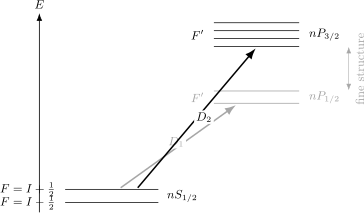
Hierarchy of the alkali resonance doublet, not to scale. Spin–orbit coupling splits the $nP$ term into $J=1/2$ and $J=3/2$ levels, while nuclear spin divides each fine-structure level into isotope-dependent hyperfine levels $F$. The arrows denote the $D_1$ and $D_2$ optical manifolds, not single two-level transitions.

Rounded wavelengths and configurations

Element	Ground configuration	Common nuclear-spin examples	Approximate $D_2$ wavelength	Representative AMO role
Li	$[\mathrm{He}]2s\,{}^2S_{1/2}$	$^6$Li: $I=1$; $^7$Li: $I=3/2$	$671\ \mathrm{nm}$	light quantum gases; fermion–boson isotope pair
Na	$[\mathrm{Ne}]3s\,{}^2S_{1/2}$	$^{23}$Na: $I=3/2$	$589\ \mathrm{nm}$	laser cooling, quantum gases, bright resonance fluorescence
K	$[\mathrm{Ar}]4s\,{}^2S_{1/2}$	$^{39}$K: $I=3/2$; $^{40}$K: $I=4$	$767\ \mathrm{nm}$	tunable quantum gases and fermionic mixtures
Rb	$[\mathrm{Kr}]5s\,{}^2S_{1/2}$	$^{85}$Rb: $I=5/2$; $^{87}$Rb: $I=3/2$	$780\ \mathrm{nm}$	laser cooling, atom interferometry, Rydberg arrays
Cs	$[\mathrm{Xe}]6s\,{}^2S_{1/2}$	$^{133}$Cs: $I=7/2$	$852\ \mathrm{nm}$	primary frequency standards, cooling, Rydberg control

The wavelengths are deliberately rounded orientation values for the neutral-atom $D_2$ resonance. A precision datum must specify isotope, hyperfine and Zeeman component, field conditions, vacuum or air wavelength, and uncertainty. Evaluated values and provenance belong in the NIST Atomic Spectra Database, not in a rounded comparison table.

Fine Structure

In a central-field picture, the leading spin–orbit contribution has the form

$$H_{\mathrm{so}}=\zeta_{n\ell}(r)\,\mathbf L\cdot\mathbf S,$$

or its radial expectation-value reduction within a chosen subshell. For a $P$ state with $L=1$ and $S=1/2$, it gives $J=1/2$ and $J=3/2$. This is the physical origin of the $D_1$–$D_2$ separation at the effective-Hamiltonian level.

The splitting generally becomes larger in heavier alkalis because the valence electron samples stronger relativistic fields. That trend is not captured reliably by inserting a screened charge into the hydrogen fine-structure formula. Core penetration, exchange, correlation, finite nuclear size, and the actual self-consistent radial orbital all matter. Precision fine-structure intervals are many-body atomic-structure observables. Fine Structure develops the relativistic operator hierarchy and the LS, jj, and intermediate-coupling limits.

The Spin–Orbit Coupling page owns the angular-momentum algebra. Here its practical role is to define the two optical resonance manifolds and their different excited-state angular structure.

Hyperfine Structure

If the nucleus has spin $I$, it couples to the electronic angular momentum $J$ to form

$$\mathbf F=\mathbf I+\mathbf J, \qquad F=|I-J|,\ldots,I+J.$$

For a weak magnetic field and a well-resolved fine-structure level, the leading magnetic-dipole constant $A$ gives an energy proportional to $\mathbf I\cdot\mathbf J$. An electric-quadrupole constant $B$ can contribute only when both the nuclear and electronic angular momenta support a rank-2 coupling. Hyperfine Structure is the canonical home for the $A$–$B$ Hamiltonian, its $F$-dependent spectrum, and the limits of the isolated-$J$ approximation.

Ground-state doublet

For the common alkali isotopes with $I\ne0$, the $nS_{1/2}$ ground state has two hyperfine levels,

$$F=I-\frac12, \qquad F=I+\frac12.$$

Their separation is a microwave frequency. It supplies long-lived internal states for clocks, interferometers, magnetometers, quantum memories, and qubit encodings. “Long lived” does not mean perfectly isolated: magnetic fields, collisions, blackbody radiation, microwave leakage, differential light shifts, and motion can all shift or decohere the transition.

The SI second is defined by fixing the unperturbed ground-state hyperfine transition frequency of caesium-133 to the exact value

$$\Delta\nu_{\mathrm{Cs}} =9\,192\,631\,770\ \mathrm{Hz}.$$

This is a definition of the unit, not the raw frequency of an atom in a laboratory. A caesium primary standard must realize the unperturbed transition by evaluating Zeeman, Stark, collisional, motional, blackbody, cavity, and interrogation shifts with uncertainties.

Magnetic fields and basis changes

At sufficiently weak field, $F$ and $m_F$ are useful labels and the first-order Zeeman shift is approximately

$$\Delta E_Z=g_F\mu_Bm_FB.$$

As the Zeeman energy becomes comparable to the hyperfine splitting, $F$ ceases to be an exact label. The eigenstates continuously approach an uncoupled $|m_I,m_J\rangle$ basis in the hyperfine Paschen–Back regime. Calculations and transition labels must use the coupling scheme appropriate to the field strength; extrapolating a low-field $g_F$ formula through an avoided crossing is not reliable. Zeeman Effect in Atoms develops the Breit–Rabi crossover and its spectroscopic consequences.

Optical Transitions Are Multilevel

At the fine-structure level, an electric-dipole transition changes parity and obeys $\Delta J=0,\pm1$, excluding $J=0\leftrightarrow J'=0$. When hyperfine structure is resolved, the corresponding angular rules include

$$\Delta F=0,\pm1, \qquad F=0\not\leftrightarrow F'=0,$$

and the polarization selects $\Delta m_F=0$ or $\pm1$ relative to the quantization axis. These statements identify angular zeros. Actual line strengths also contain reduced matrix elements, angular coefficients, state mixing, detuning, and experimental polarization geometry.

Cooling and repumping

Many alkali cooling schemes drive a nearly closed component of the $D_2$ manifold. With a suitable quantization axis and circular polarization, a stretched transition can repeatedly absorb and emit photons without immediately changing ground hyperfine level. In practice, off-resonant excitation, imperfect polarization, magnetic-field variation, and unresolved excited-state structure open leakage paths.

If spontaneous emission transfers population into the other ground hyperfine manifold, the cooling light becomes far off resonance and that population is dark. A repump laser returns it to the optical cycle. The need for repumping is not a technical afterthought; it follows directly from the multilevel branching structure.

For an idealized two-level atom, the steady scattering rate is

$$R_{\mathrm{sc}} =\frac{\Gamma}{2} \frac{s}{1+s+(2\Delta/\Gamma)^2},$$

where $\Gamma$ is the natural decay rate, $s$ the on-resonance saturation parameter, and $\Delta$ the laser detuning. The mean radiation-pressure force for a single traveling wave is $\hbar\mathbf kR_{\mathrm{sc}}$. In a real alkali atom, Clebsch–Gordan coefficients, optical pumping, several detunings, laser linewidth, and coherences modify the effective rate.

Dark states are sometimes the resource

Coherent superpositions can decouple from the applied light and form dark states. They can reduce an ordinary cooling force, but they also enable sub-Doppler cooling, electromagnetically induced transparency, coherent population trapping, and Raman control. Whether a dark state is an error or a tool depends on the intended effective Hamiltonian and dissipation channels.

Why Alkalis Are Common AMO Platforms

Several advantages coincide:

• a single valence electron gives transparent term labels and tractable calculations;
• strong $S$–$P$ resonance lines lie at wavelengths reachable with mature laser technology;
• hyperfine and Zeeman sublevels provide microwave and Raman addressability;
• several elements have multiple isotopes, including bosonic and fermionic atomic statistics;
• room-temperature vapor cells are practical for Na, K, Rb, and Cs, although useful vapor pressure and chemical handling differ strongly by species;
• strong optical cycling supports fluorescence detection and radiation-pressure forces;
• Rydberg excitation gives large, controllable dipole interactions;
• collisions and Feshbach resonances make several isotopes useful for quantum gases.

These strengths do not make alkalis universally optimal. Alkaline-earth and alkaline-earth-like atoms offer narrow intercombination and clock transitions; trapped ions provide strong confinement and excellent state detection; metastable species, molecules, and solid-state emitters support different observables. Platform choice should follow linewidth, wavelength, interaction, systematic-error, and control requirements.

Major Use Cases

Laser cooling and magneto-optical traps

Red-detuned counterpropagating beams produce velocity-dependent scattering because the Doppler shift moves an atom toward resonance with the beam opposing its motion. A magneto-optical trap adds a magnetic-field gradient and polarization pattern so that position-dependent Zeeman shifts create a restoring force as well.

A working alkali MOT requires more than the slogan “six beams plus a quadrupole field.” One must specify the isotope, cooling and repump transitions, detunings, intensities, polarization handedness relative to the field, field gradient, beam geometry, and whether the excited hyperfine structure is resolved. Lithium and potassium, whose excited-state hyperfine intervals can be small compared with optical linewidths, require different cooling strategies from a naïve resolved-level model.

The atom-specific level and polarization structure is developed in Zeeman Effect in Atoms, the operational transition rules in Atomic Selection Rules, the general perturbative method in Zeeman Effect as a Perturbation Example, and transition-rate theory in Selection Rules in Transition Rates. Laser Cooling owns the force–diffusion, capture, recoil, and thermometry framework applied to those species-specific cycles.

Microwave clocks and coherent control

Ground-hyperfine transitions are narrow because electric-dipole decay between the two levels is forbidden. Caesium-133 realizes the SI second, while rubidium standards are widely used where compactness and robustness matter. Magnetically insensitive transitions usually mean that the first derivative with respect to field vanishes at a chosen operating point, not that every magnetic contribution is zero.

Raman lasers can couple the two ground hyperfine manifolds through one or more off-resonant excited states. Eliminating those states produces an effective two-level coupling, but also AC Stark shifts and spontaneous-scattering errors. Detuning, polarization, and all relevant intermediate hyperfine paths must be treated consistently. Stark Effect in Atoms develops the scalar, vector, and tensor response and the distinction between trapping and differential shifts.

Rydberg arrays and blockade

Laser excitation to a high-$n$ state creates an atom with a large electronic orbit and strong state-dependent interactions. For two states coupled predominantly by a van der Waals interaction,

$$V(R)=\frac{C_6}{R^6}.$$

If $|V(R)|$ exceeds the excitation linewidth or Rabi scale, simultaneous excitation of nearby atoms is suppressed: this is Rydberg blockade. A common estimate of the blockade radius is

$$R_b =\left(\frac{|C_6|}{\hbar\Omega}\right)^{1/6},$$

for resonant Rabi frequency $\Omega$ in an idealized two-atom model. Real arrays must account for angular dependence, Zeeman structure, Förster resonances, motion, laser noise, finite lifetime, and inhomogeneous light shifts.

Rubidium and caesium are common because their ground and Rydberg states can be addressed with established laser systems and because state-selective fluorescence detection is efficient. The effective spin model used for an array is not the full atomic Hamiltonian; it results from choosing a small internal-state manifold and controlling leakage and dissipation.

Rydberg Atoms Basics develops the effective-$n$ scaling laws, pair-interaction regimes, blockade Hamiltonian, and many-body reduction summarized here.

Quantum-degenerate gases

Alkali isotopes supply both bosons and fermions. Bose–Einstein condensation, degenerate Fermi gases, mixtures, optical lattices, and tunable interactions have all been realized with alkalis. At ultralow temperature, electronic structure enters through effective scattering parameters and molecular bound states. A simple one-electron orbital picture does not determine the many-body phase: quantum statistics, density, trapping, multichannel collisions, and interaction tuning become the relevant variables.

Species Notes

Lithium

Lithium is light, so recoil velocities and recoil energies are comparatively large. The $^6$Li and $^7$Li isotopes provide fermionic and bosonic platforms. Its small excited-state splittings complicate a resolved-hyperfine picture of ordinary Doppler cooling, while broad interaction resonances make $^6$Li especially important for strongly interacting Fermi gases.

Sodium

Sodium’s bright yellow resonance doublet made it historically central to optical spectroscopy. The single stable isotope $^{23}$Na has $I=3/2$. Sodium supports robust laser cooling and quantum-gas experiments, but the required yellow laser wavelength has historically demanded different laser technology from the near-infrared diode systems common for Rb and Cs.

Potassium

Potassium offers several useful isotopes. The rare fermion $^{40}$K is important in degenerate Fermi gases, while $^{39}$K and $^{41}$K are bosons. The comparatively small separation within the $4P$ manifold and its hyperfine structure affects cooling and optical-pumping choices. Species labels alone are insufficient: isotope and field regime materially change the level diagram.

Rubidium

Rubidium combines accessible near-infrared D lines, two naturally occurring isotopes, convenient vapor pressure, and a large experimental literature. It is widely used in MOTs, atom interferometers, vapor-cell sensors, quantum memories, condensates, and neutral-atom Rydberg arrays. That popularity should not be confused with theoretical simplicity at precision level; transition amplitudes, polarizabilities, and clock shifts still require many-body calculations and evaluated data.

Caesium

Caesium-133 is the only stable caesium isotope and has $I=7/2$. Its ground hyperfine interval defines the second, and its relatively large fine and hyperfine splittings make several manifolds easy to resolve. Caesium is also used in fountains, interferometers, parity-violation studies, cooling experiments, and Rydberg control. Its heavy nucleus and strong relativistic effects make a nonrelativistic screened-Coulomb model inadequate for precision work.

Francium extends the sequence to still stronger relativistic and nuclear effects, but it has no stable isotope and requires radioactive-atom facilities. It is therefore scientifically important without sharing the routine experimental availability of the five species emphasized above.

Choosing the Right Model

The phrase “alkali atom” does not select a unique theoretical method. Match the model to the observable:

Target	Minimum useful description	Frequent missing physics
qualitative level ordering	central model potential with quantum defects	perturbers and channel mixing
cooling cycle	resolved fine, hyperfine, Zeeman, polarization, and decay branching	coherences, laser noise, off-resonant leakage
clock shift	field-dressed hyperfine Hamiltonian and apparatus model	collisions, blackbody shift, motion, distributed fields
transition amplitude	correlated relativistic electronic structure	core polarization, normalization, consistent effective operators
Rydberg blockade	state-resolved pair interaction plus laser coupling	anisotropy, Förster defects, motion, decay
ultracold collisions	multichannel molecular potentials and threshold scattering	three-body loss and confinement effects

Observable-level validation

A defensible calculation or data table should record:

1. isotope and nuclear spin;
2. electronic, fine-structure, hyperfine, and magnetic quantum labels appropriate to the field;
3. energy-zero and frequency convention;
4. air or vacuum wavelength and the conversion model, if a wavelength is quoted;
5. field, polarization, temperature, density, and trapping conditions that shift the datum;
6. electronic-structure method, basis or grid convergence, and treatment of core correlation;
7. source version, uncertainty, and whether values are measured, fitted, or calculated.

Agreement of energy levels does not guarantee accurate dipole matrix elements or polarizabilities. Energies, short-range hyperfine constants, long-range Rydberg defects, and transition amplitudes test different parts of an approximate wavefunction.

Common Mistakes

• Calling an alkali atom exactly hydrogenic. The $-1/r$ tail is hydrogenic; the core region, quantum defects, fine structure, and hyperfine structure are not.
• Treating the core as inert for every observable. Core polarization and virtual excitation can dominate corrections to transition amplitudes and polarizabilities.
• Interpreting a D line as one transition. It is a fine-structure manifold containing isotope-, hyperfine-, Zeeman-, and polarization-resolved components.
• Using a two-level scattering formula without a leakage model. Optical pumping and repumping are part of the physical system.
• Quoting a wavelength without its convention. Air versus vacuum, isotope, component, field, and rounding can exceed the claimed precision.
• Assuming a quantum defect is constant and universal. It belongs to a specified series, threshold, isotope, and fit convention and can vary with energy.
• Equating an exact defining frequency with an uncorrected measurement. The caesium definition refers to an unperturbed transition; a clock realizes it through a systematic-error model.
• Using low-field $F,m_F$ labels at all magnetic fields. Hyperfine and Zeeman couplings change the useful basis.
• Assuming alkalis are best for every clock or qubit. Platform virtues are observable-specific; narrow optical clocks generally favor other electronic structures.
• Reading the active-electron picture as distinguishability. The complete electronic state remains antisymmetric under exchange of any two electrons.

Exercises

1. Residual-core potential

A valence electron is at radius $r$ outside the closed-shell core of a neutral alkali atom. Use charge counting to derive the leading Coulomb potential. If the core polarizability is $\alpha_c$, find the radius at which the magnitudes of the formal terms $-1/r$ and $-\alpha_c/(2r^4)$ are equal. Why should that radius be interpreted cautiously?

Solution

If the neutral atom has nuclear charge $Z$ and $Z$ electrons, the core contains $Z-1$ electrons. Its net charge is therefore

$$Z-(Z-1)=+1.$$

The distant valence electron has potential energy $-1/r$ in atomic units. Equating the magnitudes of the Coulomb and polarization terms gives

$$\frac1r=\frac{\alpha_c}{2r^4}, \qquad r=\left(\frac{\alpha_c}{2}\right)^{1/3}.$$

This is only a comparison of asymptotic terms. If the resulting radius lies in or near the electronic core, the multipole and polarization expansion is not quantitatively valid there. Exchange, penetration, finite core size, and higher response terms then require a microscopic or fitted potential.

2. Hyperfine doublet and centroid

Consider an alkali $S_{1/2}$ level in an isotope with $I=3/2$. List the allowed $F$ values. Using only the magnetic-dipole term $E_F=AK/2$, find both energies relative to the hyperfine center of gravity and show that their separation is $2A$.

Solution

With $I=3/2$ and $J=1/2$,

$$F=|I-J|,I+J=1,2.$$

The quantity $K$ is

$$\begin{aligned} K_{F=2} &=2(3)-\frac32\frac52-\frac12\frac32 =\frac32,\\ K_{F=1} &=1(2)-\frac32\frac52-\frac12\frac32 =-\frac52. \end{aligned}$$

Hence

$$E_2=\frac{3A}{4}, \qquad E_1=-\frac{5A}{4},$$

and $E_2-E_1=2A$. The degeneracy-weighted centroid vanishes:

$$\frac{(2\cdot2+1)E_2+(2\cdot1+1)E_1}{5+3}=0.$$

This confirms that the quoted energies are measured from the unresolved fine-structure level’s center of gravity. The electric-quadrupole term vanishes because $J=1/2$.

3. Why there are two D lines

Use angular momentum and parity to explain why an alkali $nS_{1/2}$ ground state has allowed transitions to both $nP_{1/2}$ and $nP_{3/2}$. Why does this not imply that each D line is an isolated two-level transition?

Solution

For the ground state, $L=0$ and $S=1/2$, so $J=1/2$. The excited $P$ term has $L=1$ and $S=1/2$, which can couple to

$$J=\left|L-S\right|,L+S =\frac12,\frac32.$$

An electric-dipole operator changes parity and allows $\Delta J=0,\pm1$ except $0\leftrightarrow0$. Both $1/2\to1/2$ and $1/2\to3/2$ therefore survive, giving $D_1$ and $D_2$.

If $I\ne0$, each fine-structure level contains several $F$ levels and each $F$ contains $2F+1$ magnetic sublevels. Polarization, Zeeman shifts, and spontaneous-emission branching connect different subsets. The “D line” is consequently a manifold, and a two-level reduction requires specified detuning, polarization, fields, and leakage bounds.

4. Binding from illustrative quantum defects

Two Rydberg series converge to the same threshold. At $n=20$, take the illustrative defects $\delta_s=3.13$ and $\delta_f=0.02$. Find the effective principal quantum numbers and the ratio of binding-energy magnitudes in the constant-defect approximation.

Solution

The effective quantum numbers are

$$\begin{aligned} n_s^*&=20-3.13=16.87,\\ n_f^*&=20-0.02=19.98. \end{aligned}$$

Because the binding magnitude scales as $(n^*)^{-2}$,

$$\frac{|E_s-E_{\mathrm{ion}}|} {|E_f-E_{\mathrm{ion}}|} =\left(\frac{19.98}{16.87}\right)^2 \approx1.40.$$

The more strongly penetrating $s$ state is about $40\%$ more deeply bound at the same nominal $n$ in this model. The defects here are illustrative inputs, not universal alkali constants; a precision calculation would use a specified series fit and its energy dependence.

5. Why a repump is needed

A cooling laser addresses a ground hyperfine level $F=2$. The desired cycling transition reaches $F'=3$, which can decay only back to $F=2$ under the electric-dipole $\Delta F$ rule. Explain why population can nevertheless accumulate in a second ground level $F=1$, and describe the role of a repump laser.

Solution

The ideal $F=2\to F'=3$ branch is closed with respect to hyperfine decay because $F'=3\to F=1$ would have $\Delta F=-2$. Real cooling light can also excite nearby $F'=2$ through finite detuning, power broadening, imperfect polarization, or unresolved structure. That level may decay to either $F=2$ or $F=1$.

Once an atom reaches $F=1$, the cooling laser is displaced by approximately the ground hyperfine splitting and scatters very weakly. The atom becomes dark to the cooling cycle. A repump laser drives $F=1$ to an excited level that can decay into $F=2$, restoring population to the cycle. A quantitative model must include the relevant branching ratios and coherences rather than assigning a perfect closure by label alone.

Cross-Links

• Atomic Selection Rules develops electronic, hyperfine, polarization, and higher-multipole transition rules.
• Atomic Term Symbols decodes the doublet $S$, $P$, and $D$ labels used for one-valence-electron levels.
• Rydberg Atoms Basics explains high-$n$ scaling, pair interactions, and blockade.
• Atomic Physics places alkalis in the wider hierarchy of atomic models and observables.
• Atomic Units and Scales supplies the unit conventions used for effective potentials and polarizabilities.
• Hydrogen as Atomic Prototype separates reusable Coulomb structure from one-electron special cases.
• Central-Field Approximation is the canonical home for screening, shell structure, and effective orbital diagnostics.
• Fine Structure explains the relativistic kinetic, spin–orbit, Darwin, and many-electron terms behind the $D_1$–$D_2$ separation.
• Hyperfine Structure derives the nuclear dipole and quadrupole interactions, $F$ multiplets, and microwave clock intervals summarized here.
• Zeeman Effect in Atoms develops alkali magnetic-field regimes, Breit–Rabi energies, and polarization-resolved line patterns.
• Stark Effect in Atoms develops alkali static and dynamic polarizabilities, differential shifts, and trapping applications.
• Rydberg Formula develops the empirical series law that quantum defects generalize.
• Atomic Spectra Applications and Dipole Transitions develop angular factors and selection rules.
• Zeeman Effect as a Perturbation Example and Stark Effect as a Perturbation Example give canonical perturbative field-shift methods.
• AMO Physics Roadmap locates alkali spectroscopy, cooling, clocks, and Rydberg control in a longer study path.

References

1. C. J. Foot, Atomic Physics (Oxford University Press, 2005), Chapters 4–9.
2. W. R. Johnson, Atomic Structure Theory: Lectures on Atomic Physics (Springer, 2007), doi:10.1007/978-3-540-68013-0.
3. H. J. Metcalf and P. van der Straten, Laser Cooling and Trapping (Springer, 1999), doi:10.1007/978-1-4612-1470-0.
4. E. Arimondo, M. Inguscio, and P. Violino, “Experimental Determinations of the Hyperfine Structure in the Alkali Atoms,” Reviews of Modern Physics 49, 31–75 (1977), doi:10.1103/RevModPhys.49.31.
5. T. F. Gallagher, Rydberg Atoms (Cambridge University Press, 1994), doi:10.1017/CBO9780511524530.
6. M. Saffman, T. G. Walker, and K. Mølmer, “Quantum Information with Rydberg Atoms,” Reviews of Modern Physics 82, 2313–2363 (2010), doi:10.1103/RevModPhys.82.2313.
7. A. Browaeys and T. Lahaye, “Many-Body Physics with Individually Controlled Rydberg Atoms,” Nature Physics 16, 132–142 (2020), doi:10.1038/s41567-019-0733-z.
8. E. L. Raab, M. Prentiss, A. Cable, S. Chu, and D. E. Pritchard, “Trapping of Neutral Sodium Atoms with Radiation Pressure,” Physical Review Letters 59, 2631–2634 (1987), doi:10.1103/PhysRevLett.59.2631.
9. A. Kramida, Y. Ralchenko, J. Reader, and the NIST ASD Team, NIST Atomic Spectra Database, National Institute of Standards and Technology, doi:10.18434/T4W30F.
10. National Institute of Standards and Technology, Atomic Spectroscopy: Term Series and Quantum Defects.
11. National Institute of Standards and Technology, Basic Atomic Spectroscopic Data: Li, Na, K, Rb, and Cs, with associated persistent- and strong-line tables.
12. D. A. Steck, Alkali D Line Data, isotope-resolved reference sheets with stated constants, conventions, and source histories.
13. Bureau International des Poids et Mesures, SI Base Unit: Second and The International System of Units, 9th ed.