Stark Effect as a Perturbation Example

The Stark effect is the shift, splitting, and mixing of quantum levels produced by an applied electric field. As a perturbation-theory example, its central lesson is not a single formula. It is the choice among nondegenerate, degenerate, and nearly degenerate treatments after symmetry has identified which states the electric dipole can couple.

This page owns that method decision and two hydrogen checks. The compact named-effect definition belongs to Stark Effect; the field-free Coulomb spectrum belongs to Hydrogen Atom; Stark Effect in Atoms owns atom-specific DC manifolds, alkali examples, traps, and spectroscopic interpretation; and Dynamic Polarizability owns the complete frequency-dependent response.

Hamiltonian and Sign Convention

For a system with electric dipole operator $\mathbf d$ in a spatially uniform static field $\boldsymbol{\mathcal E}$,

$$H(\boldsymbol{\mathcal E}) = H_0 - \mathbf d\mathbin{\cdot}\boldsymbol{\mathcal E}.$$

Choose the field along the $z$ axis:

$$\boldsymbol{\mathcal E} = \mathcal E\,\hat{\mathbf z}, \qquad V = -\mathcal E d_z.$$

For one electron bound to a nucleus fixed at the origin, let $e\gt0$ denote the magnitude of the electron charge. Then

$$\mathbf d=-e\mathbf r,$$

so the electronic perturbation is

$$V=e\mathcal E z.$$

This sign convention matters when naming a particular oriented eigenstate. The observable set of split energies is unchanged if one reverses both the field-axis convention and the state labels.

The electric-dipole approximation also assumes that the field varies negligibly across the system. If gradients on the atomic scale matter, higher multipoles and center-of-mass forces must be included.

Symmetry Before Summation

Suppose $H_0$ is invariant under spatial inversion:

$$\mathsf P H_0\mathsf P^{-1}=H_0,$$

while

$$\mathsf P d_z\mathsf P^{-1}=-d_z.$$

It follows that

$$\mathsf P H(\mathcal E) \mathsf P^{-1} = H(-\mathcal E).$$

For an isolated nondegenerate branch that is analytic at $\mathcal E=0$, this unitary equivalence implies

$$E_n(\mathcal E)=E_n(-\mathcal E).$$

Every odd power in its small-field energy expansion therefore vanishes. In particular,

$$\Delta E_n^{(1)} = -\mathcal E \langle n\vert d_z\vert n\rangle =0.$$

This conclusion is stronger than noticing one zero integral: it constrains the whole isolated energy branch.

For central-potential orbital states, $z$ is the zero spherical component of a rank-$1$ odd-parity tensor. Its leading orbital selection rules are

$$\Delta\ell=\pm1, \qquad \Delta m=0.$$

The choice $\boldsymbol{\mathcal E}\parallel\hat{\mathbf z}$ leaves axial rotations intact, so $m$ remains a useful label in the spinless model. A field in an arbitrary direction is handled by rotating the quantization axis or by retaining all three spherical dipole components.

Degeneracy changes the parity argument. Opposite-parity states at the same unperturbed energy can be exchanged by inversion and mixed by $d_z$. Their individual energy branches may be linear and swap under $\mathcal E\mapsto-\mathcal E$, even though the spectrum as an unordered set remains field-reversal symmetric.

Which Perturbation Theory Applies?

Let $\mathcal D$ be a set of states close enough in energy to require comparison. The useful scale is not $\mathcal E$ alone but

$$v_{ab} \equiv \mathcal E \left| \langle a\vert d_z\vert b\rangle \right|.$$

Compare $v_{ab}$ with the field-free splitting

$$\delta_{ab} \equiv \left| E_a^{(0)}-E_b^{(0)} \right|.$$

Situation	Leading method	Typical energy response
isolated parity eigenstate	nondegenerate perturbation theory	quadratic
isolated state with a permanent dipole	nondegenerate perturbation theory	linear
exact opposite-parity degeneracy	diagonalize $PVP$	linear splitting
$v_{ab}$ comparable with a small $\delta_{ab}$	quasi-degenerate effective Hamiltonian	crossover
coupling comparable with gaps outside $\mathcal D$	enlarge the model space or diagonalize numerically	multilevel
oscillating or resonant field	time-dependent response	frequency dependent

A correction with a small denominator is not an unusually large success of nondegenerate perturbation theory. It is evidence that the states joined by that denominator belong in the same model space.

Isolated Levels and Polarizability

For an isolated state with no permanent dipole, the leading shift is second order:

$$\Delta E_n^{(2)} = \mathcal E^2 \sum_{m\ne n} \frac{ \left| \langle m\vert d_z\vert n\rangle \right|^2 }{ E_n^{(0)}-E_m^{(0)} }.$$

Writing

$$\Delta E_n = -\frac{1}{2} \alpha_{zz}^{(n)} \mathcal E^2 +O(\mathcal E^4)$$

defines the static polarizability component

$$\alpha_{zz}^{(n)} = 2 \sum_{m\ne n} \frac{ \left| \langle m\vert d_z\vert n\rangle \right|^2 }{ E_m^{(0)}-E_n^{(0)} }.$$

The sum denotes a complete spectral resolution. If $H_0$ has a continuum, it includes both a sum over discrete states and an integral over continuum states.

For a nondegenerate ground state, every denominator in $\alpha_{zz}^{(0)}$ is positive, so

$$\alpha_{zz}^{(0)}\ge0$$

and the quadratic energy shift is nonpositive. For an excited state, lower and higher intermediate levels contribute with opposite signs, so its static coefficient need not be positive.

The induced dipole follows from the Hellmann–Feynman Theorem:

$$\frac{\partial E_n}{\partial\mathcal E} = -\langle d_z\rangle_{\mathcal E}.$$

Consequently,

$$\langle d_z\rangle_{\mathcal E} = \alpha_{zz}^{(n)}\mathcal E +O(\mathcal E^3)$$

for an isolated parity eigenstate. The factor $1/2$ in the energy is required because the induced dipole grows from zero as the field is applied.

Second-Order Energy Corrections is the canonical home for the tensor formula, sign analysis, and continuum completeness. Here the formula is being used to decide the Stark regime.

A Two-State Crossover

An opposite-parity pair with a finite gap provides the smallest model that connects all three method choices. The ratio of its field-induced coupling to its zero-field gap determines whether the response is weakly quadratic, strongly mixed, or effectively degenerate.

Stark Shift in a Two-Level Approximation owns the exact diagonalization, mixing angle, induced dipole, two-state polarizability, and an analytic error bound for the quadratic approximation. Its central warning is simple: a small denominator is a request to enlarge the model space, not permission to trust a divergent nondegenerate correction.

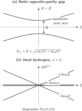
A finite opposite-parity gap produces quadratic shifts near zero field. Exact degeneracy removes that scale: in the ideal hydrogen $n=2$ manifold, two combinations split linearly while the $m=\pm1$ states have zero first-order shift.

The two-state model is the cleanest bridge between Nondegenerate Perturbation Theory, Degenerate Perturbation Theory, and Quasi-Degenerate Perturbation Theory.

Hydrogen Ground State: Exact Quadratic Check

The nonrelativistic hydrogen ground state is isolated and even under parity, so its leading DC Stark shift is quadratic. The complete sum over all opposite-parity states can be avoided with an inhomogeneous-equation method.

Use atomic units in this subsection:

$$\hbar=m_e=e=4\pi\varepsilon_0=1,$$

and neglect nuclear recoil. Then

$$\begin{aligned} H_0 &= -\frac{1}{2}\nabla^2 -\frac{1}{r}, \\ \psi_{1s} &= \frac{e^{-r}}{\sqrt\pi}, \\ E_{1s}^{(0)} &= -\frac{1}{2}. \end{aligned}$$

Write

$$\psi(\mathcal E) = \psi_{1s} + \mathcal E\chi +O(\mathcal E^2).$$

Because the perturbation is $\mathcal E z$, the first-order equation is

$$\left( H_0-E_{1s}^{(0)} \right) \chi = -z\psi_{1s}.$$

A regular solution orthogonal to $\psi_{1s}$ is

$$\chi = - \left( r+\frac{r^2}{2} \right) \cos\theta\, \psi_{1s}.$$

The second-order coefficient is then a single integral:

$$\begin{aligned} E_{1s}^{(2)} &= \langle\psi_{1s}\vert z\vert\chi\rangle \\ &= -\frac{4}{3} \int_0^\infty e^{-2r} \left( r^4+\frac{r^5}{2} \right) \,dr \\ &= -\frac{9}{4}. \end{aligned}$$

Thus, in atomic units,

$$E_{1s}(\mathcal E) = -\frac{1}{2} -\frac{9}{4}\mathcal E^2 +O(\mathcal E^4).$$

Matching to $-\alpha\mathcal E^2/2$ gives

$$\alpha_{1s} = \frac{9}{2}$$

in atomic units. In SI units, the infinite-nuclear-mass result is

$$\alpha_{1s}^{\mathrm{SI}} = \frac{9}{2} \left( 4\pi\varepsilon_0 \right) a_0^3.$$

This calculation is both a coefficient check and a completeness lesson. The inhomogeneous solution implicitly contains the discrete and continuum $p$-wave response that an explicit sum-over-states calculation must include.

Hydrogen n = 2: Degenerate Linear Effect

The ideal spinless Coulomb energy depends only on the principal quantum number $n$. The $n=2$ spatial manifold contains

$$\lvert200\rangle, \qquad \lvert210\rangle, \qquad \lvert211\rangle, \qquad \lvert21{-1}\rangle.$$

The $2s$ state $\lvert200\rangle$ is even, while the three $2p$ states are odd. With the usual real hydrogenic phases,

$$\langle200\vert z\vert210\rangle = -3a_0.$$

The $\Delta m=0$ rule removes the $m=\pm1$ states from the first-order mixing. In the ordered basis

$$\left( \lvert200\rangle, \lvert210\rangle, \lvert211\rangle, \lvert21{-1}\rangle \right),$$

the projected perturbation is

$$P_2VP_2 = e\mathcal E \begin{pmatrix} 0 & -3a_0 & 0 & 0\\ -3a_0 & 0 & 0 & 0\\ 0 & 0 & 0 & 0\\ 0 & 0 & 0 & 0 \end{pmatrix}.$$

Its first-order energy shifts are

$$\Delta E^{(1)} = +3ea_0\mathcal E, \quad -3ea_0\mathcal E, \quad 0, \quad 0.$$

The shifted states in the $m=0$ block are equal-weight combinations of $2s$ and $2p_0$. Their precise plus or minus label depends on the phase chosen for $\lvert210\rangle$; the pair of energies does not.

The linear effect is therefore not evidence that a stationary parity eigenstate had a permanent dipole before the field was applied. It comes from diagonalizing the dipole operator inside an exactly degenerate subspace. The resulting field-adapted combinations do have oriented dipole moments.

For the full ideal Coulomb shell, parabolic coordinates diagonalize the first-order Stark perturbation. The $n=2$ matrix above is the smallest explicit instance of that more general structure.

The Hydrogen Degeneracy Warning

The phrase “hydrogen has a linear Stark effect” is incomplete until the reference Hamiltonian and field scale are stated.

The ideal Coulomb Hamiltonian makes $2s$ and $2p$ exactly degenerate. Real hydrogen contains fine structure, the Lamb shift, hyperfine structure, and other smaller terms. Let $\delta$ denote the relevant zero-field splitting and let

$$v_{\mathrm{Stark}} \sim e\mathcal E \left| \langle a\vert z\vert b\rangle \right|.$$

The hierarchy determines the useful basis:

• If $v_{\mathrm{Stark}}\ll\delta$, start from the already split physical levels; their leading response can be quadratic.
• If $v_{\mathrm{Stark}}\sim\delta$, retain both the small zero-field splitting and the electric-field coupling in a quasi-degenerate matrix.
• If $\delta\ll v_{\mathrm{Stark}}$ while coupling to other principal shells remains small, the ideal degenerate-manifold linear result is a good leading description.
• If the field coupling is comparable with gaps to neighboring shells, enlarge the basis and test convergence numerically.

This ordering issue is not unique to hydrogen. Alkali quantum defects, molecular parity doublets, tunneling doublets, and hyperfine multiplets all create small denominators that can turn a nominally quadratic response into a linear or crossover regime.

Degeneracy of the Hydrogen Atom explains the accidental Coulomb degeneracy and its limits. Atomic Physics Applications maps the symmetry, coupling-scheme, and spectroscopy context without duplicating the perturbative calculation.

Uniform Fields Produce Resonances

There is a second hydrogen caveat. In the fixed-nucleus point-Coulomb model,

$$V_{\mathrm{tot}}(\mathbf r) = - \frac{e^2}{ 4\pi\varepsilon_0 r } + e\mathcal E z.$$

For every nonzero spatially uniform $\mathcal E$, this potential descends without bound in the downfield direction. The field-free bound states become metastable Stark resonances with finite ionization widths rather than exact square-integrable eigenstates.

Weak-field perturbation theory still gives highly useful real energy shifts, but its series is asymptotic and no finite order captures the exponentially small field-ionization width. The width is nonperturbative in the field near $\mathcal E=0$.

This does not invalidate ordinary low-field spectroscopy. It states the approximation honestly: the resonance lifetime must be long compared with the observation time, the field must be weak on the scale of neighboring-level mixing unless that mixing is included, and a perfectly uniform field extending to spatial infinity is an idealization.

From Level Shifts to Spectral Lines

A measured transition responds to the difference between two level shifts:

$$\hbar\,\delta\omega_{fi} = \Delta E_f-\Delta E_i.$$

Two levels can each move substantially while their transition frequency changes little, or their polarizabilities can differ enough to produce a large differential shift.

The field also changes eigenstates. To first order in an isolated case,

$$\begin{aligned} \lvert n(\mathcal E)\rangle ={}& \lvert n\rangle \\ & - \mathcal E \sum_{m\ne n} \frac{ \langle m\vert d_z\vert n\rangle }{ E_n^{(0)}-E_m^{(0)} } \lvert m\rangle \\ & +O(\mathcal E^2). \end{aligned}$$

That mixing can redistribute line strengths and weakly activate transitions forbidden at zero field. Energies alone therefore do not determine a Stark spectrum.

An oscillating field introduces detuning, absorption, and the dynamical polarizability. It belongs to Harmonic Perturbations, not to the static substitution $\mathcal E\mapsto\mathcal E(t)$ in the formulas above.

Practical Workflow

1. Write the dipole convention. State whether $e$ is signed or positive and whether $V=-\mathbf d\cdot\boldsymbol{\mathcal E}$.
2. Choose the unperturbed Hamiltonian. Decide whether fine, hyperfine, Lamb, tunneling, or crystal-field splittings belong in $H_0$.
3. Use symmetry first. Determine parity, conserved axial quantum numbers, and dipole selection rules.
4. Compare coupling with gaps. Evaluate $\mathcal E|\langle a|d_z|b\rangle|/\delta_{ab}$ for every suspicious pair.
5. Choose the model space. Use an isolated-state sum only after excluding exact and near degeneracies.
6. Include the continuum when required. A bound-state list need not be a complete basis.
7. Distinguish levels from lines. Compute differential shifts and, when needed, field-modified transition amplitudes.
8. State the field regime. Separate DC from AC response and bound-state approximations from resonance physics.

Common Mistakes

• Writing $V=-e\mathcal E z$ while also taking $e\gt0$ for an electron without explaining the sign convention.
• Concluding that every Stark effect is quadratic because diagonal dipole elements vanish in parity eigenstates.
• Applying nondegenerate second order inside the exactly degenerate hydrogen shell.
• Treating a small denominator as a trustworthy enhancement instead of enlarging the model space.
• Calling the ideal $n=2$ result the weak-field limit of real hydrogen without comparing with fine structure and the Lamb shift.
• Summing only discrete hydrogen states when calculating the exact ground-state polarizability.
• Confusing a level shift with the shift of a transition frequency.
• Replacing a static field by an oscillating field without changing to dynamical response theory.
• Describing uniform-field hydrogen levels as exact bound states at nonzero field rather than long-lived resonances.

Exercises

1. Field reversal and parity

Assume $H_0$ is inversion symmetric and $\lvert n\rangle$ is an isolated nondegenerate eigenstate. Prove that its analytic Stark energy contains only even powers of $\mathcal E$. Why does this not forbid linear splitting of an opposite-parity degenerate pair?

Solution

Because

$$\mathsf P H(\mathcal E)\mathsf P^{-1} = H(-\mathcal E),$$

the two Hamiltonians have the same spectrum. An isolated eigenvalue can be followed uniquely and continuously from $\mathcal E=0$, so

$$E_n(\mathcal E)=E_n(-\mathcal E).$$

Its Taylor series is therefore even.

At a degeneracy, a unique branch label does not exist before the perturbation is diagonalized. Parity can exchange the two field-adapted branches under $\mathcal E\mapsto-\mathcal E$. The set of eigenvalues remains symmetric even when the individual analytic branches are linear.

2. Recover the quadratic limit

Starting from the exact two-state energies, expand through order $\mathcal E^2$ for $\lvert\mathcal E d_{ab}\rvert\ll\Delta$.

Solution

Use

$$\sqrt{ \frac{\Delta^2}{4} + \mathcal E^2|d_{ab}|^2 } = \frac{\Delta}{2} \sqrt{ 1+ \frac{ 4\mathcal E^2|d_{ab}|^2 }{\Delta^2} }.$$

Expanding the square root,

$$\begin{aligned} \sqrt{ \frac{\Delta^2}{4} + \mathcal E^2|d_{ab}|^2 } ={}& \frac{\Delta}{2} \\ & + \frac{ \mathcal E^2|d_{ab}|^2 }{\Delta} \\ & +O(\mathcal E^4). \end{aligned}$$

Since $\bar E-\Delta/2=E_a^{(0)}$ and $\bar E+\Delta/2=E_b^{(0)}$,

$$\begin{aligned} E_- &= E_a^{(0)} - \frac{ \mathcal E^2|d_{ab}|^2 }{\Delta} +O(\mathcal E^4), \\ E_+ &= E_b^{(0)} + \frac{ \mathcal E^2|d_{ab}|^2 }{\Delta} +O(\mathcal E^4). \end{aligned}$$

These shifts agree with nondegenerate second order for a pair of levels coupled only to each other.

3. Diagonalize the hydrogen n = 2 block

Diagonalize the $2s$–$2p_0$ block and compute the dipole expectation value of each field-adapted state.

Solution

With

$$A=3ea_0\mathcal E,$$

the block is

$$\begin{pmatrix} 0 & -A\\ -A & 0 \end{pmatrix}.$$

Its normalized eigenstates can be chosen as

$$\begin{aligned} \lvert+\rangle &= \frac{ \lvert200\rangle+\lvert210\rangle }{\sqrt2}, \\ \lvert-\rangle &= \frac{ \lvert200\rangle-\lvert210\rangle }{\sqrt2}, \end{aligned}$$

with shifts $-A$ and $+A$, respectively, for the stated phase convention.

Because $V=-\mathcal E d_z$,

$$\Delta E^{(1)} = -\mathcal E \langle d_z\rangle.$$

The two states therefore have

$$\begin{aligned} \langle+\vert d_z\vert+\rangle &= +3ea_0, \\ \langle-\vert d_z\vert-\rangle &= -3ea_0. \end{aligned}$$

They are oriented combinations formed by the field; neither original parity eigenstate had a diagonal dipole.

4. Verify the hydrogen polarizability integral

Evaluate the radial integral in the inhomogeneous-equation calculation and recover $\alpha_{1s}=9/2$ in atomic units.

Solution

Use

$$\int_0^\infty r^n e^{-2r}\,dr = \frac{n!}{2^{n+1}}.$$

Then

$$\begin{aligned} \int_0^\infty e^{-2r} \left( r^4+\frac{r^5}{2} \right) \,dr &= \frac{4!}{2^5} + \frac{1}{2} \frac{5!}{2^6} \\ &= \frac{27}{16}. \end{aligned}$$

Therefore

$$E_{1s}^{(2)} = -\frac{4}{3} \frac{27}{16} = -\frac{9}{4}.$$

Comparing $E_{1s}^{(2)}\mathcal E^2$ with $-\alpha_{1s}\mathcal E^2/2$ gives

$$\alpha_{1s}=\frac{9}{2}.$$

5. Discrete versus continuum response

Why does a sum over only the discrete excited hydrogen states fail to reproduce the exact $1s$ polarizability? What can be said about its sign error if the retained states are exact?

Solution

The Coulomb Hamiltonian has both discrete bound states and a continuum above ionization. Completeness in the dipole response requires both:

$$\begin{aligned} \alpha_{zz}^{(0)} ={}& 2\sum_{\mathrm{bound}} \frac{ |\langle m|d_z|0\rangle|^2 }{ E_m-E_0 } \\ & + 2\int_{\mathrm{cont}} \frac{ |\langle E|d_z|0\rangle|^2 }{ E-E_0 } \,dE. \end{aligned}$$

For the ground state, every denominator is positive. Omitting exact continuum contributions therefore makes the result too small, not too large. This monotonic statement need not survive arbitrary approximate pseudostates or inconsistent normalization.

6. Differential Stark shift

Two isolated nondegenerate levels have no permanent dipoles and static polarizabilities $\alpha_i$ and $\alpha_f$. Find the leading shift of their transition angular frequency and state when it vanishes.

Solution

Each level shifts by

$$\Delta E_j = -\frac{1}{2} \alpha_j\mathcal E^2 +O(\mathcal E^4).$$

Hence

$$\delta\omega_{fi} = - \frac{ \alpha_f-\alpha_i }{ 2\hbar } \mathcal E^2 +O(\mathcal E^4).$$

The leading transition shift vanishes when the two static polarizabilities are equal, even though each level can have a nonzero Stark shift.

Cross-Links

• Stark Effect in Atoms for atom-specific polarizabilities, AC shifts, trapping, and spectroscopy.
• Time-Independent Perturbation Theory for the chapter-level decision framework.
• Stark Shift in a Two-Level Approximation for the exact finite-gap crossover, induced dipole, and quadratic-error estimate.
• Second-Order Energy Corrections for polarizability and signed denominator sums.
• Degenerate Perturbation Theory for projected first-order diagonalization.
• Quasi-Degenerate Perturbation Theory for finite small splittings.
• Hellmann–Feynman Theorem for induced dipoles as energy derivatives.
• Hydrogen Atom for the field-free wavefunctions and spectrum.
• Degeneracy of the Hydrogen Atom for the enlarged Coulomb symmetry.
• Selection Rules for the tensor and parity logic.
• Atomic Physics Applications for the symmetry and spectroscopy map.
• Stark Effect for the compact named-effect entry.

References

• J. Stark, “Observation of the Separation of Spectral Lines by an Electric Field,” Nature 92, 401 (1913), doi:10.1038/092401b0.
• J. Stark, “Beobachtungen über den Effekt des elektrischen Feldes auf Spektrallinien. I. Quereffekt,” Annalen der Physik 348, 965–982 (1914), doi:10.1002/andp.19143480702.
• E. Schrödinger, “Quantisierung als Eigenwertproblem. Dritte Mitteilung: Störungstheorie, mit Anwendung auf den Starkeffekt der Balmerlinien,” Annalen der Physik 385, 437–490 (1926), doi:10.1002/andp.19263851302.
• A. Dalgarno and J. T. Lewis, “The Exact Calculation of Long-Range Forces between Atoms by Perturbation Theory,” Proceedings of the Royal Society A 233, 70–74 (1955), doi:10.1098/rspa.1955.0246.
• I. W. Herbst and B. Simon, “Stark Effect Revisited,” Physical Review Letters 41, 67–69 (1978), doi:10.1103/PhysRevLett.41.67.
• A. Hooker, C. H. Greene, and W. Clark, “Classical Examination of the Stark Effect in Hydrogen,” Physical Review A 55, 4609–4612 (1997), doi:10.1103/PhysRevA.55.4609.
• H. A. Bethe and E. E. Salpeter, Quantum Mechanics of One- and Two-Electron Atoms, Springer, 1957.
• C. Cohen-Tannoudji, B. Diu, and F. Laloë, Quantum Mechanics, Vol. II, Wiley, 1977.
• L. D. Landau and E. M. Lifshitz, Quantum Mechanics: Non-Relativistic Theory, 3rd ed., Pergamon, 1977.