Zeeman Effect as a Perturbation Example

The Zeeman effect is the shift and splitting of quantum levels in an applied magnetic field. As a perturbation-theory example, its main lesson is that weak field is not a complete prescription. One must say which internal interaction defines the unperturbed basis, which zero-field levels are degenerate, and how the magnetic energy compares with fine-structure, hyperfine, and neighboring electronic gaps.

This page owns that method choice and a solvable crossover model. The historical discovery and the normal-versus-anomalous story belong to Zeeman Effect Revisited; magnetic-moment and $g$-factor conventions belong to Magnetic Moments and g-Factors; and atomic Landé patterns, Breit–Rabi energies, polarization, and spectroscopic inference belong to Zeeman Effect in Atoms.

Magnetic-Field Hamiltonian

For a magnetic moment operator $\boldsymbol\mu$ in a static field $\mathbf B$, the magnetic-dipole interaction is

$$H_Z=-\boldsymbol\mu\mathbin{\cdot}\mathbf B.$$

This compact formula hides two issues that matter in perturbation theory:

• the magnetic moment may contain orbital, spin, nuclear, and relativistic contributions;
• minimal coupling also produces a term quadratic in the field.

Consider one electron of charge $-e$, with $e\gt0$, bound to a fixed nucleus. In the symmetric gauge for a uniform field,

$$\mathbf B=B\hat{\mathbf z}, \qquad \mathbf A=\frac12\mathbf B\mathbin{\times}\mathbf r.$$

The nonrelativistic Hamiltonian, including the electron spin magnetic moment, is

$$H = \frac{(\mathbf p+e\mathbf A)^2}{2m_e} +V(\mathbf r) +\frac{g_s\mu_B}{\hbar}\mathbf S\mathbin{\cdot}\mathbf B,$$

where

$$\mu_B=\frac{e\hbar}{2m_e}$$

is the Bohr magneton and $g_s\simeq2.002319$ for a free electron. Expanding in powers of $B$ gives

$$H(B)=H_0+B\mathcal M_z+B^2\mathcal D,$$

with

$$\mathcal M_z = \frac{\mu_B}{\hbar} \left(L_z+g_sS_z\right)$$

and

$$\mathcal D = \frac{e^2}{8m_e} \left(x^2+y^2\right).$$

Equivalently,

$$\begin{aligned} H(B) ={}&H_0 +\frac{\mu_BB}{\hbar} \left(L_z+g_sS_z\right) \\ &+ \frac{e^2B^2}{8m_e} \left(x^2+y^2\right). \end{aligned}$$

The term linear in $B$ is commonly called the paramagnetic or Zeeman term. The explicit $B^2$ term is diamagnetic. For many electrons, $\mathbf L$ and $\mathbf S$ in the leading linear term are sums over the electrons. Nuclear magnetic moments add terms on the scale of the nuclear magneton and therefore introduce a separate, usually smaller, hierarchy.

The derivation and gauge interpretation of the orbital term are developed at Orbital Magnetic Moments. Here the expansion is the starting point for choosing a perturbative regime.

What Counts as a Small Field?

A field is small only relative to specified energy gaps. Useful ratios include

$$\begin{aligned} \epsilon_{mathrm{fs}} &= \frac{\mu_BB}{\Delta_{mathrm{fs}}}, \\ \epsilon_{mathrm{el}} &= \frac{\mu_BB}{\Delta_{mathrm{el}}}, \end{aligned}$$

where $\Delta_{mathrm{fs}}$ is a relevant fine-structure separation and $\Delta_{mathrm{el}}$ is a gap to a different electronic term. If hyperfine structure is resolved, one also needs

$$\epsilon_{mathrm{hfs}} = \frac{\mu_BB}{\Delta_{mathrm{hfs}}}.$$

These ratios answer different questions. A field may be strong enough to decouple $\mathbf L$ and $\mathbf S$ while remaining far too weak to mix different electronic configurations. Likewise, a field can overwhelm hyperfine coupling while leaving fine structure almost untouched.

For a spatial orbital of characteristic transverse size $a_\perp$, a rough comparison of the explicit diamagnetic term with an electronic gap is

$$\epsilon_{mathrm{dia}} \sim \frac{e^2B^2a_\perp^2}{8m_e\Delta_{mathrm{el}}}.$$

Calling a field weak without recording the relevant ratios leaves the approximation undefined.

Symmetry Before Diagonalization

A uniform magnetic field is an axial vector. The leading Zeeman operator is even under spatial inversion, so parity remains a useful label when $H_0$ is parity invariant:

$$\mathsf P H(B)\mathsf P^{-1}=H(B).$$

Full rotational symmetry is reduced to rotations about the field axis. Consequently, a magnetic projection such as $M$, $m_J$, or $m_L+m_S$ remains conserved in the appropriate model even when $J$ itself does not.

Time reversal gives a subtler diagnostic. At zero field,

$$\Theta\mathbf L\Theta^{-1}=-\mathbf L, \qquad \Theta\mathbf S\Theta^{-1}=-\mathbf S.$$

Therefore the field-dependent family obeys

$$\Theta H(B)\Theta^{-1}=H(-B).$$

If an isolated zero-field eigenvalue is nondegenerate and maps back to the same analytic branch under time reversal, then

$$E_n(B)=E_n(-B),$$

so its linear coefficient vanishes. This does not forbid the familiar linear Zeeman effect. Rotational multiplets are degenerate, and half-integer-spin systems with time-reversal symmetry have Kramers pairs. Time reversal can exchange the split branches:

$$E_+(B)=E_-(-B),$$

while each branch separately has a nonzero slope at $B=0$.

This is a useful general lesson: a symmetry can constrain the set of eigenvalues without making every branch an even function of the perturbation.

Degenerate First-Order Splitting

Let $P$ project onto a zero-field eigenspace of $H_0$ with energy $E_0$. The first-order problem is not the list of diagonal matrix elements in an arbitrary basis. It is the projected operator

$$W=P\mathcal M_zP.$$

Its eigenvalues $w_a$ determine the linear branches,

$$E_a(B)=E_0+Bw_a+O(B^2),$$

and its eigenvectors give the combinations selected by the field. Only after diagonalizing $W$ may one use ordinary nondegenerate formulas on separated branches.

Spinless orbital multiplet

For a central spinless problem with fixed orbital angular momentum $\ell$,

$$W=\frac{\mu_B}{\hbar}L_z.$$

The $L_z$ basis already diagonalizes the projected perturbation:

$$\Delta E_{ell m_\ell}^{(1)} = \mu_BB,m_\ell, \qquad m_\ell=-\ell,\ldots,\ell.$$

The field resolves the $(2\ell+1)$-fold multiplet into an equally spaced fan. Its first-order center of gravity is unchanged because

$$\sum_{m_\ell=-\ell}^{\ell}m_\ell=0.$$

This vanishing trace is basis independent:

$$\operatorname{tr}_{P}(W)=0.$$

It says that the linear perturbation redistributes levels around the original centroid; it does not say that individual levels are unshifted.

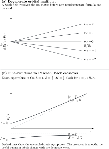
Two distinct uses of degenerate or quasi-degenerate perturbation theory. (a) The $m_\ell$ basis resolves a degenerate orbital multiplet immediately. (b) When the Zeeman and spin–orbit scales compete, fixed-$M$ blocks must be diagonalized; coupled $J$ labels evolve continuously into uncoupled $(m_L,m_S)$ labels.

Weak-Field LS Coupling

Suppose electrostatic interactions and spin–orbit coupling have already produced levels labeled by

$$\lvert \alpha L S J M_J\rangle,$$

where $\alpha$ denotes any remaining quantum numbers. The weak-field condition is schematically

$$\mu_BB\ll\Delta_{mathrm{fs}},$$

so mixing between distinct $J$ levels may be neglected at first order. The field still splits the degenerate $M_J$ states inside a fixed $J$ multiplet.

Within that multiplet, the projection theorem makes the vector operators $\mathbf L$ and $\mathbf S$ proportional to $\mathbf J$. Their diagonal matrix elements are

$$\begin{aligned} \langle L_z\rangle &=\hbar M_J C_L, \\ \langle S_z\rangle &=\hbar M_J C_S, \end{aligned}$$

where

$$\begin{aligned} C_L &= \frac12 + \frac{L(L+1)-S(S+1)}{2J(J+1)}, \\ C_S &= \frac12 + \frac{S(S+1)-L(L+1)}{2J(J+1)}. \end{aligned}$$

The coefficients satisfy $C_L+C_S=1$, as they must because $J_z=L_z+S_z$.

The first-order shift becomes

$$\Delta E_{alpha LSJM_J}^{(1)} = g_J\mu_BB M_J,$$

where

$$g_J = g_LC_L+g_sC_S.$$

For the leading electronic orbital moment, $g_L=1$. The formula assumes $J\ne0$; an isolated $J=0$ level has no first-order electronic Zeeman shift within that one-dimensional subspace, although second-order mixing and nuclear contributions may remain.

The angular-momentum derivation and convention ledger are canonical at Magnetic Moments and g-Factors. The perturbative point here is that $g_J$ is a projected weak-field coefficient, not a universal constant valid after different $J$ manifolds begin to mix.

A doublet P term

Take $L=1$, $S=1/2$, $g_L=1$, and approximate $g_s=2$. The two fine-structure levels have

$$g_{3/2}=\frac43, \qquad g_{1/2}=\frac23.$$

Thus the weak-field branches are

$$\Delta E^{(1)} = g_J\mu_BB M_J.$$

For example, the $M_J=1/2$ slopes are $2\mu_B/3$ for $J=3/2$ and $\mu_B/3$ for $J=1/2$. Those two branches will reappear in the exact crossover model below.

Weak, Intermediate, and Strong-Field Bases

The labels that simplify the problem depend on the ordering of terms in the Hamiltonian.

Regime	Scale hierarchy	Useful leading basis	Required calculation
Weak Zeeman relative to fine structure	$\mu_BB\ll\Delta_{\mathrm{fs}}$	$\lvert \alpha LSJM_J\rangle$	Project into a fixed $J$ multiplet; use $g_JM_J$
Intermediate field	$\mu_BB\sim\Delta_{\mathrm{fs}}$	Fixed-$M$ basis spanning several $J$ values	Diagonalize spin–orbit plus Zeeman terms together
Paschen–Back regime	$\Delta_{\mathrm{fs}}\ll\mu_BB\ll\Delta_{\mathrm{el}}$	$\lvert \alpha Lm_L\rangle\lvert Sm_S\rangle$	Treat spin–orbit coupling as the smaller term
Diamagnetic high-field regime	Orbital $B^2$ term or inter-term mixing is appreciable	Problem dependent	Retain minimal coupling beyond the linear Zeeman model

In the Paschen–Back regime, the leading electronic shift is

$$\Delta E \simeq \mu_BB\left(m_L+g_sm_S\right).$$

The inequality on the right of the Paschen–Back hierarchy matters: the field may dominate spin–orbit coupling while remaining a perturbation relative to the electronic binding and configuration gaps. Once the diamagnetic term and broad orbital reorganization compete with those scales, the simple phrase “strong-field Zeeman effect” is no longer a controlled model.

Hyperfine structure introduces another crossover. At the weakest fields, states may be labeled by $\mathbf F=\mathbf I+\mathbf J$ and $m_F$. When the electronic and nuclear Zeeman terms compete with the hyperfine splitting, one diagonalizes fixed-$m_F$ blocks; at larger fields, $m_J$ and $m_I$ become more useful. This hyperfine Paschen–Back crossover is distinct from the decoupling of $\mathbf L$ and $\mathbf S$. See Coupling Schemes for the broader hierarchy.

Exact Two-State Crossover

A two-dimensional block makes the change of basis explicit. Consider

$$H = \frac{A}{\hbar^2}\mathbf L\mathbin{\cdot}\mathbf S + \frac{\mu_BB}{\hbar} \left(L_z+2S_z\right),$$

with $L=1$, $S=1/2$, and $A\gt0$. Define

$$x=\mu_BB.$$

The conserved projection is

$$M=m_L+m_S.$$

In the $M=1/2$ subspace, choose the uncoupled basis

$$\lvert a\rangle = \lvert m_L=0,m_S=1/2\rangle,$$ $$\lvert b\rangle = \lvert m_L=1,m_S=-1/2\rangle.$$

Using

$$\mathbf L\mathbin{\cdot}\mathbf S = L_zS_z +\frac12\left(L_+S_-+L_-S_+\right),$$

the Hamiltonian block is

$$H_{M=1/2} = \begin{pmatrix} x & A/\sqrt2 \\ A/\sqrt2 & -A/2 \end{pmatrix}.$$

The exact eigenvalues are

$$\begin{aligned} E_\pm(x) ={}& \frac{x}{2}-\frac{A}{4} \\ &\pm \sqrt{ \left(\frac{x}{2}+\frac{A}{4}\right)^2 +\frac{A^2}{2} }. \end{aligned}$$

At zero field,

$$E_+(0)=\frac{A}{2}, \qquad E_-(0)=-A,$$

which are the $J=3/2$ and $J=1/2$ fine-structure energies. Their initial slopes are

$$\left.\frac{dE_+}{dx}\right|_{x=0}=\frac23, \qquad \left.\frac{dE_-}{dx}\right|_{x=0}=\frac13,$$

in agreement with $g_JM_J$.

For $x\gg A$,

$$E_+(x)=x+O\!\left(\frac{A^2}{x}\right),$$

and

$$E_-(x) = -\frac{A}{2} +O\!\left(\frac{A^2}{x}\right).$$

The corresponding eigenvectors approach $\lvert a\rangle$ and $\lvert b\rangle$. Nothing discontinuous happens to the states. What changes is which approximate quantum number makes the dominant Hamiltonian nearly diagonal.

The example is also a warning about fixed-basis perturbation series. Expanding around $x=0$ is useful for $x/A\ll1$; expanding around the uncoupled basis is useful for $A/x\ll1$; and neither asymptotic description is uniformly accurate through the crossover. Direct block diagonalization is the natural intermediate-field method.

Quadratic Zeeman Shifts

Suppose a nondegenerate branch of $H_0$ is sufficiently isolated and write

$$H(B)=H_0+B\mathcal M_z+B^2\mathcal D.$$

Through second order in $B$,

$$\begin{aligned} E_n(B) ={}& E_n^{(0)} +B(\mathcal M_z)_{nn} \\ &+B^2\left(\mathcal D_{nn}+Q_n\right) +O(B^3). \end{aligned}$$

Here

$$Q_n = \sum_{m\ne n} \frac{ \lvert(\mathcal M_z)_{mn}\rvert^2 }{E_n^{(0)}-E_m^{(0)}},$$

with $(\mathcal M_z)_{mn}=\langle m\rvert\mathcal M_z\lvert n\rangle$ and $\mathcal D_{nn}=\langle n\rvert\mathcal D\lvert n\rangle$.

There are therefore two conceptually distinct quadratic contributions:

1. the expectation value of the explicit diamagnetic operator $\mathcal D$;
2. virtual mixing generated twice by the linear magnetic operator $\mathcal M_z$.

If the first-order coefficient vanishes by symmetry, these terms often provide the leading shift. Near a small denominator, however, the sum is a warning that the allegedly nondegenerate state should be enlarged into a quasi-degenerate model space.

For a branch that emerged from a degenerate eigenspace, first diagonalize $P\mathcal M_zP$. The quadratic formula must then be applied to those field-selected zeroth-order combinations, with any remaining degeneracy treated explicitly.

Levels Versus Spectral Lines

The Zeeman Hamiltonian shifts levels. Spectroscopy measures differences between an upper level $u$ and a lower level $\ell$. In the weak-field LS regime,

$$\hbar\,\delta\omega_{u\ell} = \mu_BB \left( g_uM_u-g_\ell M_\ell \right).$$

Electric-dipole transitions have magnetic selection rule

$$\Delta M=0,\pm1,$$

subject to the remaining angular-momentum selection rules. The $\Delta M=0$ components are conventionally called $\pi$ components, and the $\Delta M=\pm1$ components $\sigma^\pm$ components. Their observed polarization depends on viewing geometry.

The familiar three-component normal Zeeman pattern is a special case in which the upper and lower level shifts combine into only three distinct transition frequencies. Generic anomalous patterns contain more components because $g_u$ and $g_\ell$ differ and because several magnetic sublevels participate. Level counting alone does not determine line strengths; those require dipole matrix elements and angular-momentum coefficients.

A Reliable Workflow

1. Write the complete field dependence needed at the intended order. Distinguish the linear magnetic-dipole term from the explicit diamagnetic term.
2. List the zero-field energy scales. Include hyperfine, fine-structure, electronic, and any accidental near-degeneracy gaps that can compete with $\mu_BB$.
3. Identify exact symmetries at fixed field. Parity and the projection along $\mathbf B$ often survive even when $J$ does not.
4. Choose the model space. Include every state connected by the perturbation whose separation is comparable to the relevant coupling.
5. Diagonalize inside that space. Use $P H_ZP$, or diagonalize spin–orbit plus Zeeman terms together when neither is small relative to the other.
6. Treat the complement perturbatively. Estimate corrections using coupling-to-gap ratios rather than the field magnitude alone.
7. Translate level shifts into observables. Form transition-energy differences and then apply selection rules and line-strength factors.
8. State the regime with the result. A formula labeled only “Zeeman shift” is incomplete.

Common Mistakes

• Taking diagonal matrix elements in an arbitrary degenerate basis. The eigenvalues of $P H_ZP$, not its displayed diagonal entries, are the first-order shifts.
• Using the Landé factor outside weak LS coupling. Once different $J$ levels mix substantially, $g_JM_J$ is not an exact label for the branch.
• Forgetting the electron-sign convention. The electron magnetic moment is antiparallel to its angular momentum, while the standard electronic energy shift is written with positive $\mu_B(L_z+g_sS_z)/\hbar$.
• Dropping the $B^2$ term automatically. It is higher order near $B=0$, but can dominate a symmetry-forbidden linear shift or become nonperturbative at high field.
• Calling every strong-field limit Paschen–Back. Paschen–Back means decoupling of specified angular momenta while the field remains small relative to larger electronic scales.
• Confusing hyperfine and fine-structure crossovers. Decoupling $\mathbf I$ from $\mathbf J$ and decoupling $\mathbf L$ from $\mathbf S$ occur at different field scales.
• Equating level splitting with a spectral triplet. Transition frequencies depend on both levels, and intensities require transition matrix elements.
• Assuming time reversal forbids linear splitting. It makes an isolated nondegenerate branch even in $B$; it can exchange two branches of a degenerate multiplet.

Exercises

Recover the orbital and diamagnetic terms

For an electron in the symmetric gauge $\mathbf A=\mathbf B\times\mathbf r/2$, expand $(\mathbf p+e\mathbf A)^2/(2m_e)$ and show that the field-dependent orbital terms are

$$\frac{\mu_B}{\hbar}\mathbf B\mathbin{\cdot}\mathbf L + \frac{e^2}{8m_e} \lvert\mathbf B\mathbin{\times}\mathbf r\rvert^2.$$

Solution

Expand the square with operator ordering retained:

$$\begin{aligned} (\mathbf p+e\mathbf A)^2 ={}& \mathbf p^2 +e\mathbf p\mathbin{\cdot}\mathbf A \\ &+e\mathbf A\mathbin{\cdot}\mathbf p +e^2\mathbf A^2. \end{aligned}$$

The symmetric gauge obeys $\boldsymbol\nabla\mathbin{\cdot}\mathbf A=0$, so

$$\mathbf p\mathbin{\cdot}\mathbf A = \mathbf A\mathbin{\cdot}\mathbf p.$$

Moreover,

$$\mathbf A\mathbin{\cdot}\mathbf p = \frac12 (\mathbf B\mathbin{\times}\mathbf r) \mathbin{\cdot}\mathbf p = \frac12\mathbf B\mathbin{\cdot}\mathbf L.$$

Therefore

$$\mathcal C \equiv \frac{e}{2m_e} (\mathbf p\mathbin{\cdot}\mathbf A +\mathbf A\mathbin{\cdot}\mathbf p).$$

Using the two identities above,

$$\begin{aligned} \mathcal C &= \frac{e}{m_e} \mathbf A\mathbin{\cdot}\mathbf p \\ &= \frac{e}{2m_e} \mathbf B\mathbin{\cdot}\mathbf L \\ &= \frac{\mu_B}{\hbar} \mathbf B\mathbin{\cdot}\mathbf L. \end{aligned}$$

Finally,

$$\frac{e^2\mathbf A^2}{2m_e} = \frac{e^2}{8m_e} \lvert\mathbf B\mathbin{\times}\mathbf r\rvert^2.$$

Split an orbital quintet

A spinless $\ell=2$ level has zero-field energy $E_0$. Find its first-order orbital Zeeman energies and verify that their centroid remains $E_0$.

Solution

The five magnetic quantum numbers are

$$m_\ell=-2,-1,0,1,2.$$

Thus

$$E_{m_\ell}(B) = E_0+\mu_BB m_\ell+O(B^2).$$

The average first-order shift is

$$\frac{\mu_BB}{5} \sum_{m_\ell=-2}^{2}m_\ell=0.$$

The centroid is unchanged through first order even though four of the five branches move linearly.

Reconcile time reversal with linear splitting

Explain why a nondegenerate spinless level has no linear Zeeman shift at $B=0$ when time reversal is a symmetry, while a degenerate pair can split as $E_0\pm cB$.

Solution

The Hamiltonian family satisfies

$$\Theta H(B)\Theta^{-1}=H(-B).$$

For an isolated nondegenerate branch, time reversal must map the state back to the same branch up to phase, so

$$E(B)=E(-B).$$

Its Taylor series contains only even powers of $B$ near zero.

For a degenerate pair, time reversal may exchange the two field-selected eigenstates. The constraint is then

$$E_+(B)=E_-(-B),$$

which is satisfied by

$$E_\pm(B)=E_0\pm cB+O(B^2).$$

Degenerate perturbation theory determines $c$ from the eigenvalues of the projected magnetic operator.

Evaluate two Landé factors

For $L=1$, $S=1/2$, $g_L=1$, and $g_s=2$, calculate $g_J$ for $J=3/2$ and $J=1/2$. Then give the slopes of the $M_J=1/2$ branches with respect to $B$.

Solution

The projection coefficients obey $C_L+C_S=1$. Since $g_L=1$ and $g_s=2$,

$$g_J = C_L+2C_S = 1+C_S,$$

where

$$C_S = \frac12 + \frac{S(S+1)-L(L+1)}{2J(J+1)}.$$

one obtains

$$g_{3/2}=\frac43, \qquad g_{1/2}=\frac23.$$

Because

$$\frac{dE}{dB}=g_J\mu_BM_J,$$

the $M_J=1/2$ slopes are

$$\left.\frac{dE}{dB}\right|_{J=3/2,M_J=1/2} = \frac23\mu_B,$$

and

$$\left.\frac{dE}{dB}\right|_{J=1/2,M_J=1/2} = \frac13\mu_B.$$

Diagonalize the crossover block

Diagonalize

$$H= \begin{pmatrix} x & A/\sqrt2 \\ A/\sqrt2 & -A/2 \end{pmatrix}$$

and check both the $x=0$ energies and the $x\gg A$ limits.

Solution

For a symmetric matrix

$$\begin{pmatrix} a&v\\ v&d \end{pmatrix},$$

the eigenvalues are

$$\frac{a+d}{2} \pm \sqrt{ \left(\frac{a-d}{2}\right)^2+v^2 }.$$

Here $a=x$, $d=-A/2$, and $v=A/\sqrt2$, giving

$$E_\pm = \frac{x}{2}-\frac{A}{4} \pm \sqrt{ \left(\frac{x}{2}+\frac{A}{4}\right)^2 +\frac{A^2}{2} }.$$

At $x=0$, the square root is $3A/4$, so

$$E_+(0)=\frac{A}{2}, \qquad E_-(0)=-A.$$

For $x\gg A$, expanding the square root gives

$$E_+(x)=x+O(A^2/x),$$ $$E_-(x)=-\frac{A}{2}+O(A^2/x).$$

The eigenstates therefore approach the two uncoupled basis vectors that diagonalize the dominant Zeeman term.

Obtain the normal triplet

Consider a spinless electric-dipole transition from an upper $\ell=1$ level to a lower $\ell=0$ level. Ignore the quadratic shift. Show that the allowed transition frequencies form three equally spaced components.

Solution

The lower level has only $m_\ell=0$ and therefore no linear orbital shift. The upper level has

$$\Delta E_u=\mu_BB m_\ell, \qquad m_\ell=-1,0,1.$$

The electric-dipole rule $\Delta m_\ell=0,\pm1$ allows all three upper substates to connect to the lower state. If $\omega_0$ is the zero-field transition frequency, then

$$\omega_{m_\ell} = \omega_0 +\frac{\mu_BB}{\hbar}m_\ell.$$

The three components lie at

$$\omega_0-\frac{\mu_BB}{\hbar}, \qquad \omega_0, \qquad \omega_0+\frac{\mu_BB}{\hbar}.$$

This equal triplet is special. Different upper and lower Landé factors generally produce a more complicated anomalous pattern.

Cross-Links

• Time-Independent Perturbation Theory
• Degenerate Perturbation Theory
• Quasi-Degenerate Perturbation Theory
• Second-Order Energy Corrections
• Zeeman Effect in Atoms
• Zeeman Effect Revisited
• Zeeman Effect
• Magnetic Moments and g-Factors
• Spin in Magnetic Fields
• Orbital Magnetic Moments
• Coupled and Uncoupled Bases
• Coupling Schemes
• Atomic Physics Applications
• Selection Rules

References

• P. Zeeman, “The effect of magnetisation on the nature of light emitted by a substance,” Philosophical Magazine 43, 226–239, 1897.
• F. Paschen and E. Back, “Normale und anomale Zeemaneffekte,” Annalen der Physik 344, 897–932, 1912.
• A. Landé, “Termstruktur und Zeemaneffekt der Multipletts,” Zeitschrift für Physik 15, 189–205, 1923.
• G. Breit and I. I. Rabi, “Measurement of nuclear spin,” Physical Review 38, 2082–2083, 1931.
• C. J. Foot, Atomic Physics, Oxford University Press, 2005.
• C. Cohen-Tannoudji, B. Diu, and F. Laloë, Quantum Mechanics, Vol. 2, Wiley, 1977.
• J. J. Sakurai and J. Napolitano, Modern Quantum Mechanics, 3rd ed., Cambridge University Press, 2020.
• I. I. Sobelman, Atomic Spectra and Radiative Transitions, 2nd ed., Springer, 1992.