Worked Problems and Model Calculations

A worked problem should do more than display algebra. It should make every scientific choice visible: what is being predicted, why a method is appropriate, which scale controls the approximation, how the result is checked, and where the conclusion stops being trustworthy.

This chapter collects canonical model calculations built around that full chain. General proofs and reusable formulas remain on the method pages. Exact model definitions remain in their canonical-system homes. Numerical algorithms and convergence studies belong in the computational notebooks. The worked pages connect those layers around a specific question.

The governing workflow is

$$\begin{gathered} \text{model and observable} \\ \downarrow \\ \text{regime and method} \\ \downarrow \\ \text{calculation and validation} \\ \downarrow \\ \text{qualified claim}. \end{gathered}$$

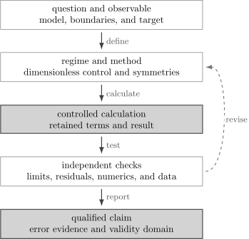
A model calculation is complete only after the result survives checks that are not built into the approximation itself. A failed check sends the calculation back to its scale analysis or method choice; it should not be hidden by adding digits.

What Every Worked Problem Contains

Each calculation in this chapter follows the same nine-part standard.

1. Problem statement. Specify the Hamiltonian or evolution equation, the physical preparation, the boundary conditions, and the requested observable.
2. Method choice. Explain why perturbation theory, a variational estimate, WKB, an effective Hamiltonian, or a scattering construction matches the question.
3. Assumptions and small parameter. Identify dimensionless ratios, scale separations, symmetries, and excluded regimes.
4. Calculation. Carry out enough intermediate work that signs, factors, normalizations, and approximations can be audited.
5. Result. State the answer with its dimensions and convention.
6. Validity discussion. Estimate omitted effects and name the conditions under which the answer should be trusted.
7. Cross-checks. Test limits, symmetries, normalization, conservation laws, and alternative representations.
8. Exact or numerical comparison. Use an independent benchmark when one is available.
9. Related pages. Link back to the canonical derivations and forward to broader applications.

The Error-Estimate Checklist is the final audit for items 3, 6, 7, and 8.

How to Study a Worked Calculation

The most useful order is not to read from top to bottom passively.

First read the problem statement and stop before the method choice. Decide what the observable is and list the scales. Ask which exact structure is available and which dimensionless ratio could organize an approximation.

Next compare your method choice with the page. A different method is not necessarily wrong. A quartic oscillator, for example, supports perturbative, variational, semiclassical, and numerical questions. The correct choice depends on whether the target is a weak-coupling energy coefficient, a one-sided ground-state bound, a high-lying spectrum, or a benchmark over a finite coupling range.

Then reproduce one structural step without looking: a matrix element, Fourier transform, matching condition, or dimensionless rescaling. This exposes convention mistakes faster than copying every line.

Finally inspect the validity and cross-check sections before trusting the numerical result. A calculation that agrees with your algebra but fails a known limit has not been independently verified.

Thirteen Comparison Paths

The present chapter begins with thirteen model families chosen because each admits a clean independent benchmark.

Weakly anharmonic spectra

Anharmonic Oscillator by Perturbation Theory derives first- and second-order shifts for a quartic perturbation. It links operator selection rules to a concrete asymptotic expansion and compares the truncated series with numerical diagonalization.

Anharmonic Oscillator by Variational Methods optimizes a Gaussian width, proves the resulting upper bound, and follows the same approximation from weak coupling to the pure-quartic scaling regime.

The canonical method pages are Nondegenerate Perturbation Theory and Second-Order Energy Corrections. Perturbation Theory Benchmarks owns the basis-truncation study.

This model is useful because several ideas can be separated cleanly:

• the perturbative coefficients are analytic;
• parity sharply restricts intermediate states;
• the exact finite-coupling spectrum can be approximated numerically;
• the weak-coupling series is useful without being convergent at fixed positive coupling;
• a variational estimate asks a different question from a perturbative coefficient.

Static field mixing

Stark Shift in a Two-Level Approximation exactly diagonalizes an opposite-parity pair in a uniform static electric field. The exact result supplies its own perturbative benchmark: it identifies the dimensionless mixing ratio, recovers the quadratic polarizability, and gives a closed error formula for the weak-field approximation.

Stark Effect as a Perturbation Example owns the broader symmetry decision, hydrogen calculations, continuum response, and spectroscopy caveats. Two-State Hamiltonians owns the reusable matrix algebra.

This path separates three statements that are often conflated:

• a finite opposite-parity gap produces an even, quadratic response sufficiently close to zero field;
• exact degeneracy requires diagonalization inside the degenerate subspace and produces dipole-labeled linear branches;
• exact treatment of the retained pair does not control leakage into omitted states.

Swept avoided crossings

Landau–Zener Transition Worked Example follows a two-level avoided crossing from its fixed diabatic basis to its moving adiabatic basis. It evaluates the exact asymptotic transition law, checks its exponent in complex time, and compares it with direct finite-window propagation of the Schrödinger equation.

Landau–Zener Transition owns the reusable probability formula. Adiabatic Approximation as a Method owns the general moving-basis workflow and leakage estimates.

This path is designed to expose three independent convention choices:

• whether the quoted probability tracks adiabatic or diabatic labels;
• whether the named slope belongs to one diagonal entry or their difference;
• whether the named gap is the off-diagonal coupling or the full minimum splitting.

Smooth-well spectra

WKB Bound States in a Smooth Potential evaluates the action integral of the pure quartic oscillator, derives its $E_n\propto(n+1/2)^{4/3}$ spectrum, and compares the first eight levels with converged numerical diagonalization.

Bohr–Sommerfeld Quantization owns the general action rule and Turning Points and Connection Formulas owns its Airy-matching phase. WKB Versus Exact Spectrum owns the systematic quadratic-plus-quartic coupling sweep.

This path separates three layers of the result:

• dimensional scaling fixes the powers of $\lambda$, $m$, and $\hbar$ exactly;
• the beta-function action fixes the leading semiclassical coefficient;
• numerical diagonalization measures the approximation error without assuming that WKB is variational.

Barrier transmission

WKB Barrier Tunneling Worked Example compares a semiclassical transmission exponent with the exact opaque-barrier limit. The calculation separates the robust exponential dependence from a prefactor that is more sensitive to abrupt boundaries and matching assumptions.

Barrier Penetration and Tunneling owns the general WKB derivation. The exact rectangular-barrier solution belongs to Rectangular Barrier Tunneling, while WKB Versus Exact Spectrum develops numerical comparison for bound-state quantization.

This path teaches a recurring lesson: an approximation can capture a dominant exponent accurately while leaving an order-one relative uncertainty in the prefactor. The error statement must say which part of the answer is controlled.

Nonperturbative doublets

Double-Well Splitting fixes one quartic double-well convention and follows its lowest doublet through an exact two-state Hamiltonian, a finite-energy WKB action, the analytic Euclidean instanton, and symmetry-resolved numerical diagonalization.

Tunneling Splittings owns the general quantitative dictionary, while Double-Well Tunneling owns the physical model and Instantons in Quantum Mechanics owns the reusable Euclidean saddle construction.

This path makes three nonperturbative distinctions explicit:

• perturbation theory within either well fixes a common energy but cannot generate the exponentially small gap;
• the splitting is linear in a tunneling amplitude, whereas a transmission probability is quadratic;
• agreement on the action does not by itself establish agreement on the prefactor.

Zero-range scattering

Delta Potential Scattering solves a point interaction exactly and then audits the result in lead and parity-channel conventions. Attraction and repulsion have identical reflection and transmission probabilities but opposite phase motion and different analytic continuations.

Scattering from a Delta Potential owns the elementary matching derivation, while Delta-Function Potential owns the direct bound-state solution. One-Dimensional Scattering Revisited owns the general channel dictionary and Bound States and Scattering Poles owns the analytic classification.

This path turns one solvable denominator into four independent checks:

• current conservation fixes $R+T=1$;
• the reduced even-channel eigenvalue stays on the unit circle for real $k$;
• the attractive pole reproduces the exact bound-state energy;
• its residue recovers the normalization of the bound-state tail.

Finite-range partial waves

Square-Well Scattering solves the attractive spherical well in every angular-momentum channel. One interface formula yields the exact phase shifts, the $s$-wave scattering length, and a near-threshold $p$-wave shape resonance.

Phase Shifts owns the general channel interpretation, Scattering Length owns the threshold parameter, and Resonances owns the general quasibound-state classification. Phase Shift Extraction turns the same matching logic into a numerical workflow for smooth potentials.

This path makes four checks visible in one model:

• zero potential gives $\delta_\ell=0$ in every channel;
• real matching keeps $|S_\ell|=1$;
• finite-$k$ extraction converges to the exact zero-energy scattering length;
• the $p$-wave peak saturates its partial-wave unitarity bound.

Impenetrable-core scattering

Hard-Sphere Scattering turns a Dirichlet boundary at $r=R$ into exact phase shifts for every partial wave. It derives $a=R$ and $r_e=2R/3$, compares the low-energy quantum result with classical specular reflection, and follows the exact sum toward the high-energy diffraction limit.

Partial-Wave Cross Sections owns the general channel sum, Scattering Length owns the threshold definition, and Optical Theorem owns the forward-amplitude identity behind the diffraction contribution.

This path distinguishes three areas that are easily conflated:

• coherent low-energy $s$-wave scattering gives $4\pi R^2$;
• classical impact-parameter counting gives $\pi R^2$;
• high-energy quantum reflection plus forward diffraction gives $2\pi R^2$.

Weak potential scattering

Gaussian Potential in the Born Approximation turns a potential into a scattering amplitude through a three-dimensional Fourier transform. The Gaussian model makes the transform analytic, keeps the interaction short-ranged, and exposes the momentum-transfer dependence directly.

First Born Approximation owns the general formula and Validity of the Born Approximation owns its control criteria. Phase Shift Extraction supplies an independent radial-equation benchmark.

This path separates three questions that are often blurred:

• whether the Fourier transform was calculated correctly;
• whether the chosen normalization gives the correct dimensions;
• whether repeated scattering is weak enough for first order to approximate the physical amplitude.

Screened long-range scattering

Yukawa Potential in the Born Approximation starts from $g e^{-\mu r}/r$ and derives its differential, total, and momentum-transfer cross sections. It then translates the same result into partial-wave phases, a threshold scattering length, and the static massive-exchange denominator.

Coulomb Scattering owns the unscreened long-range problem, while QFT Bridge: Born Approximation and Tree Level owns the normalization dictionary between a potential and a relativistic amplitude.

This path makes four limiting statements precise:

• finite screening regulates the Born forward amplitude;
• high momentum narrows the angular distribution without changing its fixed-parameter forward value;
• the zero-screening limit reproduces Rutherford scattering at fixed nonzero angle but not a finite total cross section;
• an attractive threshold pole invalidates first order even though the Fourier transform remains analytic.

Universal threshold scattering

Low-Energy S-Wave Scattering tunes an attractive spherical square well to $a=10R$ and compares its exact $s$-wave amplitude with the scattering-length and effective-range approximations. The calculation separates the threshold plateau, the near-unitary window, and the range-sensitive regime, then continues the same approximations to a shallow bound-state pole.

This path makes the approximation hierarchy quantitative: the scattering length fixes the universal leading behavior, the effective range extends the accurate momentum window, and the exact effective-range function exposes where both truncations cease to be controlled.

Resonance identification

Resonance from a Square Well takes the exact $p$-wave feature of the spherical well and asks whether one isolated pole controls it. A background-aware Breit–Wigner fit is compared with the exact outgoing-wave pole, while the phase crossing, unitarity-fraction peak, cross-section maximum, half-maximum width, and pole energy are kept distinct.

This path is a compact audit of resonance language: it shows what can be read from real-axis data, what depends on a fit model, and what requires analytic continuation.

Choosing a Starting Problem

Goal	Learn	Primary Check
Practice ladder-operator perturbation theory	Anharmonic oscillator	parity channels and numerical diagonalization
Compare a variational bound across coupling regimes	Variational anharmonic oscillator	upper bound, virial identity, and residual
Estimate a smooth-well spectrum from a classical action	Quartic WKB bound states	dimensional scaling and converged diagonalization
Diagnose quadratic versus linear static response	Two-level Stark shift	exact diagonalization and omitted-state audit
Connect a spectral doublet with a Euclidean saddle	Double-well splitting	parity blocks, WKB action, and instanton exponent
Compare adiabatic following with direct propagation	Landau–Zener transition	basis dictionary, window convergence, and norm
See how an exponent survives imperfect prefactors	WKB barrier	exact opaque-barrier limit
Connect exact matching with poles and residues	Delta scattering	flux, parity phases, and bound-state normalization
Connect radial matching with threshold and shape resonances	Square-well scattering	phase branches, scattering length, and unitarity
Compare wave, ray, and diffraction cross sections	Hard-sphere scattering	boundary phases, channel cutoff, and three area limits
Convert a potential into an angular distribution	Gaussian Born scattering	units, forward limit, and phase shifts
Connect screening, transport, and static exchange	Yukawa Born scattering	Fourier normalization, partial-wave sum, and screening limits
Test scattering-length universality and range corrections	Low-energy s-wave scattering	exact effective-range function, unitarity window, and shallow pole
Connect a phase-shift peak with a complex pole	Square-well resonance	background-aware fit, peak definitions, and outgoing pole
Learn to choose among methods first	Approximation Decision Tree	observable and control parameter
Audit a completed approximation	Error-Estimate Checklist	omitted terms and independent benchmarks

A Hierarchy of Cross-Checks

Cross-checks have different logical strength. Use more than one level when practical.

Exact structural checks

Dimensions, Hermiticity, normalization, symmetry, and conservation laws can rule out an answer without knowing the exact numerical solution. These checks are cheap and should be performed first.

Solvable limits

Turn off the perturbation, take a high- or low-energy limit, restore a symmetry, or approach a regime with a known exact result. A correct formula should reduce smoothly unless the limit is known to be singular.

Alternative analytic methods

Compare methods only where their regimes overlap. Perturbation theory and a variational estimate can agree at weak coupling, WKB and exact matching can agree in an opaque-barrier limit, and a Born amplitude can agree with small phase shifts. Agreement outside a shared regime may be accidental.

Independent numerics

A numerical benchmark should solve the original model rather than discretize the approximation being tested. It must also pass its own grid, basis, domain-size, and tolerance checks. Numerical convergence and approximation accuracy are separate entries in the error budget.

Experimental comparison

Data test the model, its parameters, and the approximation together. Disagreement does not identify which layer failed without a separate uncertainty analysis. Agreement after fitting several free parameters is weaker evidence than a parameter-free prediction.

Canonical Homes

Worked pages own the complete calculation for the named model and observable. They do not take ownership of every ingredient they use.

• General theorems, recursions, and approximation formulas belong to the corresponding method chapters.
• Exact spectra, wavefunctions, and elementary matching problems belong to Wave Mechanics and Model Systems.
• Symmetry algebra and selection rules belong to Symmetry, Angular Momentum, and Spin.
• Numerical algorithms, parameter sweeps, and reproducibility metadata belong to Computational Notebooks.
• Compact notation and reporting checks belong to the reference pages.

When a calculation needs one of those ingredients, it states the convention and links to the canonical derivation rather than reproducing it.

Common Mistakes

• Choosing a method before stating the observable.
• Calling a dimensional coefficient “small” without dividing by a relevant scale.
• Reproducing a general proof inside every model calculation.
• Comparing two approximations that share the same uncontrolled assumption and calling the agreement independent.
• Reporting numerical digits before checking basis, grid, or domain convergence.
• Treating a good energy estimate as evidence that every property of the wavefunction is accurate.
• Hiding a failed limit or conservation check inside a broad statement of “reasonable agreement.”

Exercises

1. Separate model, method, and observable

For a quartic oscillator, classify each item as a model choice, a method choice, or an observable: the coupling $\lambda$, Rayleigh–Ritz diagonalization, the ground-state energy, even parity, and a Gaussian trial family.

Solution

The coupling $\lambda$ and parity symmetry are parts of the model. Rayleigh–Ritz diagonalization and a Gaussian trial family are method choices, with the trial family specifying a variational approximation space. The ground-state energy is the observable. Parity also constrains which method implementations are admissible, but it is not itself an approximation.

2. Design an independent check

You derive a first Born cross section and then evaluate the same Born integral with two different quadrature routines. Is their agreement an independent test of the Born approximation? Name a stronger check.

Solution

The two quadratures test numerical evaluation of the same first-order formula. They do not test the neglect of repeated scattering. A stronger check is to compute the second Born contribution, solve the radial Schrödinger equation and extract phase shifts, or compare with an exact scattering solution for a solvable potential in an overlapping regime.

3. Report a qualified result

A WKB calculation reproduces the exact tunneling exponent but misses the exact prefactor by a factor of two. Write a scientifically accurate one-sentence conclusion.

Solution

The WKB result correctly captures the leading exponential suppression in the opaque-barrier regime, while its prefactor is only accurate to order unity for this abruptly varying barrier.

Cross-Links

• Volume Overview
• Choosing a Method
• Small Parameters and Error Estimates
• Common Failure Modes
• Method Comparison Table
• Error-Estimate Checklist
• Anharmonic Oscillator by Variational Methods
• Stark Shift in a Two-Level Approximation
• Landau–Zener Transition Worked Example
• Delta Potential Scattering
• Square-Well Scattering
• Hard-Sphere Scattering
• Yukawa Potential in the Born Approximation
• Low-Energy S-Wave Scattering
• Resonance from a Square Well
• Perturbation Theory Benchmarks
• WKB Versus Exact Spectrum
• Phase Shift Extraction

References

• R. Shankar, Principles of Quantum Mechanics, 2nd ed., Springer, 1994.
• J. J. Sakurai and J. Napolitano, Modern Quantum Mechanics, 3rd ed., Cambridge University Press, 2020.
• C. M. Bender and S. A. Orszag, Advanced Mathematical Methods for Scientists and Engineers, Springer, 1999.
• J. R. Taylor, Scattering Theory: The Quantum Theory of Nonrelativistic Collisions, Dover, 2006.
• L. N. Trefethen and D. Bau III, Numerical Linear Algebra, SIAM, 1997.