Double-Well Splitting

This worked example follows one symmetric quartic double well through four mutually checking descriptions:

1. a physical Hamiltonian and its dimensionless semiclassical parameter;
2. an exact two-state representation of the lowest even–odd doublet;
3. a WKB estimate from the energy-dependent barrier action;
4. an instanton estimate from a finite-action Euclidean trajectory.

The calculation ends with symmetry-resolved numerical diagonalization across a range of barrier depths. That comparison matters because the tunneling exponent is robust, while order-one prefactors require more care.

Double-Well Tunneling is the canonical home for the physical model. Tunneling Splittings owns the general dictionary among localized states, Herring flux, WKB, instantons, and spectral gaps. This page owns one convention-fixed hand calculation. Double-Well Instanton Numerical Check owns the downloadable solver, full convergence sweeps, independent finite-difference check, and retained data.

Problem Statement

Consider

$$\begin{aligned} H_{\mathrm{phys}} &= -\frac{\hbar^2}{2m} \frac{d^2}{dx^2} \\ &\quad+ \lambda \left( x^2-a^2 \right)^2. \end{aligned}$$

Here $\lambda\gt0$.

The minima are at $x=\pm a$, and the central barrier has height

$$V(0)=\lambda a^4.$$

For the lowest doublet, determine:

• the effective left–right Hamiltonian;
• the even–odd splitting $\Delta E$;
• the WKB barrier exponent;
• the Euclidean instanton and its action;
• the regime in which these semiclassical descriptions agree with the spectrum.

The observable is a closed-system energy difference,

$$\Delta E \equiv E_{\mathrm{odd}} - E_{\mathrm{even}} \gt0.$$

It is not a transmission probability and not a decay width.

Put the Model in Semiclassical Form

Set

$$q=\frac{x}{a}, \qquad E=2\lambda a^4\,\epsilon,$$

and define

$$g \equiv \frac{ \hbar }{ a^3\sqrt{2m\lambda} }.$$

The stationary Schrödinger equation becomes

$$H_g\psi(q) = \epsilon\psi(q),$$

with

$$\begin{aligned} H_g &= -\frac{g^2}{2} \frac{d^2}{dq^2} + U(q), \\ U(q) &= \frac12 \left( q^2-1 \right)^2. \end{aligned}$$

All dependence on $m$, $\lambda$, $a$, and $\hbar$ is now carried by the energy scale $2\lambda a^4$ and the dimensionless parameter $g$.

The dimensionless barrier height is $1/2$. Near either minimum,

$$U''(\pm1)=4,$$

so the classical small-oscillation frequency is

$$\omega_0=2.$$

Because $g$ plays the role of an effective Planck constant, the local ground energy is

$$\epsilon_{\mathrm{loc}} = \frac{g\omega_0}{2} + O(g^2) = g+O(g^2).$$

The deep-well regime is therefore

$$g\ll1,$$

where the intrawell scale $g\omega_0=2g$ is small compared with the barrier height, and the splitting is exponentially smaller still.

In physical variables, the exponent obtained below is

$$\frac{4}{3g} = \frac{ 4a^3\sqrt{2m\lambda} }{ 3\hbar }.$$

It grows with barrier width, stiffness, and square root of the mass.

Local Well Expansion

Write $q=1+y$ near the right minimum. The potential is

$$U(1+y) = 2y^2 + 2y^3 + \frac12y^4.$$

The quadratic term gives $\omega_0=2$. Ordinary perturbation theory about this local oscillator gives

$$\epsilon_{\mathrm{loc}} = g - \frac14g^2 + O(g^3).$$

The $O(g^2)$ coefficient combines the first-order quartic correction and the second-order cubic correction. This is an intrawell expansion: every finite order is the same in the left and right wells and therefore cannot by itself produce their exponentially small difference.

That distinction is central:

• finite powers of $g$ contribute to the common intrawell energy;
• the nonanalytic factor $e^{-4/(3g)}$ produces the even–odd splitting.

Perturbation theory around one minimum and tunneling semiclassics answer different parts of the spectrum.

Two-State Effective Hamiltonian

Let $\lvert e\rangle$ and $\lvert o\rangle$ denote the exact lowest even and odd eigenstates, with energies $\epsilon_e$ and $\epsilon_o$. Define orthonormal left- and right-localized combinations by

$$\begin{aligned} \lvert L\rangle &= \frac{ \lvert e\rangle+\lvert o\rangle }{ \sqrt2 }, \\ \lvert R\rangle &= \frac{ \lvert e\rangle-\lvert o\rangle }{ \sqrt2 }. \end{aligned}$$

Within this exact two-dimensional spectral subspace,

$$H_{\mathrm{eff}} = \begin{pmatrix} \bar\epsilon & -J\\ -J & \bar\epsilon \end{pmatrix} = \bar\epsilon I - J\sigma_x,$$

where

$$\bar\epsilon = \frac{ \epsilon_e+\epsilon_o }{2}, \qquad J = \frac{ \epsilon_o-\epsilon_e }{2} \gt0.$$

The sign convention $J\gt0$ makes the nodeless even state the lower state:

$$\begin{aligned} \epsilon_e &= \bar\epsilon-J, \\ \epsilon_o &= \bar\epsilon+J. \end{aligned}$$

Therefore

$$\Delta\epsilon \equiv \epsilon_o-\epsilon_e = 2J.$$

The matrix identity is exact after the doublet has been selected. Calling $\lvert L\rangle$ and $\lvert R\rangle$ spatially localized is accurate only when the doublet is well isolated and $g$ is small enough that the two lobes overlap weakly.

Coherent Transfer Between Wells

In dimensionless real time $s$, the Schrödinger equation is

$$ig \frac{d}{ds} \lvert\psi(s)\rangle = H_{\mathrm{eff}} \lvert\psi(s)\rangle.$$

Starting in $\lvert L\rangle$,

$$P_R(s) = \left| \langle R\vert\psi(s)\rangle \right|^2 = \sin^2 \left( \frac{Js}{g} \right).$$

The first complete transfer occurs at

$$s_{\mathrm{transfer}} = \frac{\pi g}{2J} = \frac{\pi g}{\Delta\epsilon}.$$

An exponentially small spectral splitting therefore means an exponentially long coherent transfer time. This oscillation is a closed-system consequence of the doublet; it should not be interpreted as a sequence of stochastic barrier crossings.

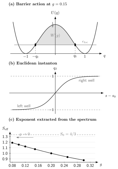
Top: at $g=0.15$, the local ground energy lies below the barrier and the one-way WKB action spans the inner turning points. Middle: the finite-action Euclidean solution $q_I(s)=\tanh(s-s_0)$ connects the two minima. Bottom: the scaled logarithm extracted from numerical gaps tends toward the instanton action $S_0=4/3$ as $g\to0$.

WKB Barrier Action

For a local level at energy $\epsilon_{\mathrm{loc}}\lt1/2$, the two inner turning points solve

$$U(q_t)=\epsilon_{\mathrm{loc}}.$$

Using the leading local energy $\epsilon_{\mathrm{loc}}=g$ gives

$$q_t(g) = \sqrt{ 1-\sqrt{2g} }, \qquad 0\lt g\lt\frac12.$$

The forbidden interval relevant to the splitting is $-q_t\lt q\lt q_t$. Its one-way action is

$$\begin{aligned} W(g) &= \int_{-q_t}^{q_t} \sqrt{ 2\left[ U(q)-g \right] } \,dq \\ &= 2 \int_0^{q_t} \sqrt{ \left( 1-q^2 \right)^2 - 2g } \,dq. \end{aligned}$$

The elementary leading connection formula for the ground doublet is

$$\Delta\epsilon_{\mathrm{WKB}} = \frac{ g\omega_0 }{\pi} \exp \left[ -\frac{W(g)}{g} \right].$$

Since $\omega_0=2$,

$$\Delta\epsilon_{\mathrm{WKB}} = \frac{2g}{\pi} e^{-W(g)/g}.$$

This formula uses the leading harmonic local energy and the leading connection prefactor consistently. Replacing $g$ in the turning-point equation by $g-g^2/4$ changes the exponent at relative algebraic order. Such a refinement can be useful, but combining it with an uncorrected prefactor is only a partial next-order calculation and need not improve the error monotonically.

Worked value at g = 0.15

For $g=0.15$,

$$q_t = \sqrt{ 1-\sqrt{0.30} } = 0.672514\ldots,$$

and numerical quadrature gives

$$W(0.15) = 0.8502476075\ldots.$$

Therefore

$$\Delta\epsilon_{\mathrm{WKB}} = 3.2980134\times10^{-4}.$$

The converged numerical splitting is

$$\Delta\epsilon_{\mathrm{num}} = 2.9960349\times10^{-4},$$

so this leading WKB estimate is about $10.1\%$ high.

Zero-energy limit

As $g\to0$, the inner turning points approach $\pm1$ and

$$\begin{aligned} W(0) &= \int_{-1}^{1} \left( 1-q^2 \right) \,dq \\ &= \frac43. \end{aligned}$$

This is the leading tunneling exponent. It is not safe to insert $W(0)=4/3$ into the energy-dependent WKB formula while keeping its original prefactor and call the result a normalized next-order estimate. Endpoint contributions migrate between exponent and prefactor when $\epsilon_{\mathrm{loc}}=O(g)$ is taken to zero.

Instanton Calculation

The dimensionless Euclidean action is

$$S_E[q] = \int ds \left[ \frac12 \left( \frac{dq}{ds} \right)^2 + U(q) \right],$$

and a path contributes with weight $e^{-S_E/g}$.

The Euclidean equation of motion is

$$\frac{d^2q}{ds^2} = \frac{dU}{dq} = 2q \left( q^2-1 \right).$$

For a trajectory satisfying

$$q(-\infty)=-1, \qquad q(+\infty)=1,$$

the first integral has zero Euclidean energy:

$$\frac12 \left( \frac{dq}{ds} \right)^2 = U(q).$$

For the increasing trajectory,

$$\frac{dq}{ds} = 1-q^2.$$

Integration gives the instanton

$$q_I(s) = \tanh \left( s-s_0 \right),$$

where $s_0$ is an arbitrary center. Translation invariance in Euclidean time makes $s_0$ a collective coordinate and produces a zero mode in the fluctuation operator.

The action is

$$\begin{aligned} S_0 &= \int_{-1}^{1} \sqrt{ 2U(q) } \,dq \\ &= \int_{-1}^{1} \left( 1-q^2 \right) \,dq \\ &= \frac43. \end{aligned}$$

Thus a one-instanton process carries the nonperturbative factor

$$e^{-S_0/g} = e^{-4/(3g)}.$$

This is the same limiting action found from WKB.

One-Loop Instanton Prefactor

The determinant calculation and zero-mode normalization belong to Fluctuation Determinants Preview. In the present Hamiltonian convention, their one-loop result gives the off-diagonal coupling

$$J_{\mathrm{inst}} = \sqrt{ \frac{32g}{\pi} } e^{-4/(3g)} \left[ 1+O(g) \right].$$

The spectral splitting is twice the coupling:

$$\Delta\epsilon_{\mathrm{inst}} = 4 \sqrt{ \frac{8g}{\pi} } e^{-4/(3g)} \left[ 1+O(g) \right].$$

Three pieces of this formula have different origins:

• $4/3$ is the classical instanton action;
• $g^{1/2}$ comes from Gaussian fluctuations and the translation zero mode;
• the factor of $2$ converts the one-instanton left–right coupling into the even–odd spectral gap.

At $g=0.15$,

$$\Delta\epsilon_{\mathrm{inst}} = 3.4094183\times10^{-4},$$

about $13.8\%$ above the numerical gap. The error is consistent with omitted relative $O(g)$ corrections; the one-loop formula is asymptotic, not exact at finite $g$.

Numerical Diagonalization

This section summarizes the spectral audit needed to close the worked calculation. The computational notebook gives the complete implementation, extends the sweep to $g=0.06$, varies $N$ and $\Omega$ independently, and records the floating-point plateau for the smallest gaps.

Use harmonic-oscillator basis states with adjustable frequency $\Omega$. With effective Planck constant $g$,

$$q = \sqrt{ \frac{g}{2\Omega} } \left( a+a^\dagger \right),$$

and

$$H_\Omega = g\Omega \left( N+\frac12 \right).$$

The quartic Hamiltonian matrix is assembled as

$$H_g = H_\Omega + \frac12 \left( q^2-I \right)^2 - \frac12\Omega^2q^2.$$

Because $U(q)$ is even, the matrix connects only basis states of the same parity. The lowest even and odd eigenvalues can therefore be found in separate blocks, avoiding accidental mixing of a nearly degenerate pair.

The table used $\Omega=2$ and $N=220$ basis states. Repeating the calculation with $N=160$, and with $\Omega=1.5$ and $3$, changed every displayed gap by less than $6\times10^{-14}$ in absolute value. This is small enough to resolve the $g=0.08$ gap to better than one part in a million.

The WKB column uses $\epsilon_{\mathrm{loc}}=g$ in the inner turning points. The instanton column uses the normalized one-loop formula above.

$g$	$W(g)$	$\Delta\epsilon_{\mathrm{num}}$	$\Delta\epsilon_{\mathrm{WKB}}$	$\Delta\epsilon_{\mathrm{inst}}$
0.30	0.464049	$2.95206\times10^{-2}$	$4.06651\times10^{-2}$	$4.10575\times10^{-2}$
0.25	0.587933	$1.19615\times10^{-2}$	$1.51522\times10^{-2}$	$1.54086\times10^{-2}$
0.20	0.716260	$3.01756\times10^{-3}$	$3.54463\times10^{-3}$	$3.63286\times10^{-3}$
0.15	0.850248	$2.99603\times10^{-4}$	$3.29801\times10^{-4}$	$3.40942\times10^{-4}$
0.12	0.934162	$2.99115\times10^{-5}$	$3.17846\times10^{-5}$	$3.30466\times10^{-5}$
0.10	0.991985	$3.01409\times10^{-6}$	$3.13145\times10^{-6}$	$3.26917\times10^{-6}$
0.08	1.051681	$9.78792\times10^{-8}$	$9.94791\times10^{-8}$	$1.04312\times10^{-7}$

The pattern is systematic:

• the WKB ratio $\Delta\epsilon_{\mathrm{WKB}}/\Delta\epsilon_{\mathrm{num}}$ falls from $1.38$ at $g=0.30$ to $1.016$ at $g=0.08$;
• the one-loop instanton ratio falls from $1.39$ to $1.066$ over the same range;
• both methods capture more than five orders of magnitude of suppression;
• neither finite-$g$ prefactor should be judged from the exponent alone.

The slightly better performance of the displayed WKB formula at the smallest $g$ is model- and convention-specific. It uses the finite local energy inside the barrier action, thereby retaining some effects that appear as algebraic corrections when the instanton result is organized around the zero-energy action.

Extract the Exponent Without Fitting the Prefactor

Suppose

$$\Delta\epsilon \sim C\sqrt g\, e^{-S_0/g}.$$

Define

$$S_{\mathrm{eff}}(g) \equiv -g \log \left( \frac{ \Delta\epsilon_{\mathrm{num}} }{ \sqrt g } \right).$$

Then

$$S_{\mathrm{eff}}(g) = S_0 - g\log C + O(g^2),$$

so

$$\lim_{g\to0} S_{\mathrm{eff}}(g) = \frac43.$$

The numerical values increase from $0.876$ at $g=0.30$ to $1.190$ at $g=0.08$, approaching $4/3$ from below. Convergence in this scaled logarithm is intentionally slow because the prefactor contributes an $O(g)$ term. The raw splitting converges much more dramatically on a logarithmic scale.

Splitting Versus Transmission

The wavefunction amplitude crossing the central barrier scales as

$$\mathcal A_{\mathrm{barrier}} \sim e^{-W/g}.$$

The doublet splitting is linear in the induced off-diagonal coupling:

$$\Delta\epsilon \sim e^{-W/g}.$$

A scattering transmission probability would square an amplitude:

$$T \sim e^{-2W/g}.$$

Using $e^{-2W/g}$ for the double-well splitting is therefore a factor-of-two error in the exponent. Boundary conditions decide whether the barrier action enters an amplitude, a probability, a spectral gap, or a decay rate.

Physical Scaling

Restoring units,

$$\Delta E = 2\lambda a^4 \Delta\epsilon.$$

At leading exponential order,

$$\Delta E \propto \exp \left[ - \frac{ 4a^3\sqrt{2m\lambda} }{ 3\hbar } \right].$$

This immediately gives three useful trends:

• increasing the separation $2a$ suppresses the gap exponentially as $a^3$ for this quartic family;
• increasing the mass suppresses the gap exponentially as $\sqrt m$;
• increasing $\lambda$ raises the local frequency but suppresses tunneling through the stronger $\sqrt\lambda$ action.

The last point warns against reasoning from an attempt frequency alone. A stiffer well produces faster local motion and a more opaque barrier; in the semiclassical regime the exponential wins.

Validity Audit

Isolated doublet

The two-state picture requires

$$\Delta\epsilon \ll g\omega_0 = 2g.$$

At $g=0.30$ the ratio is about $0.049$, already separated but not deeply asymptotic. At $g=0.08$ it is about $6.1\times10^{-7}$.

Energy below the barrier

The leading local ground energy $g$ must lie below $1/2$. The condition $g\lt1/2$ also keeps the inner turning points real. Quantitative semiclassics needs the stronger condition $g\ll1$.

Dilute instantons

The instanton width in $s$ is order unity, while the characteristic separation between tunneling events grows as $e^{S_0/g}$. A dilute instanton gas is therefore controlled when $S_0/g\gg1$.

Prefactor order

Agreement of $S_0=4/3$ proves agreement at leading exponential order. It does not prove that WKB endpoint matching and an instanton determinant have been normalized consistently. A prefactor claim must state its Hamiltonian convention and loop order.

Numerical resolution

Resolving $\Delta\epsilon$ requires absolute eigenvalue errors much smaller than the gap. Convergence of the individual energies is not enough if two nearly equal numbers are subtracted. Parity blocks, basis variation, and sufficient arithmetic precision are part of the calculation.

Coherent closed dynamics

The transfer formula assumes an isolated closed doublet. Environmental dephasing, dissipation, a static bias, or coupling to higher states changes the dynamics even if the underlying symmetric splitting remains well defined.

Common Mistakes

• Calling $\Delta\epsilon$ a tunneling probability.
• Using the transmission exponent $e^{-2W/g}$ instead of the amplitude exponent $e^{-W/g}$.
• Forgetting that the spectral gap is $2J$, not $J$.
• Mixing physical and dimensionless energies without the factor $2\lambda a^4$.
• Treating $q=0$ as an ordinary minimum rather than the barrier top.
• Expanding around one well and expecting a finite power series in $g$ to produce $e^{-4/(3g)}$.
• Replacing the finite-energy WKB action by $S_0$ while retaining an unrelated prefactor.
• Quoting an instanton determinant without specifying the normalization of $g$ and $H_g$.
• Calling the numerical gap converged after checking only the individual eigenvalues.
• Assuming localized left and right states remain stationary; the exact stationary states have definite parity.

Exercises

1. Derive the dimensionless coupling

Starting from $H_{\mathrm{phys}}$, set $x=aq$ and divide the equation by $2\lambda a^4$. Show that the kinetic term becomes $-(g^2/2)d^2/dq^2$ with

$$g = \frac{ \hbar }{ a^3\sqrt{2m\lambda} }.$$

Solution

The kinetic term transforms as

$$-\frac{\hbar^2}{2m} \frac{d^2}{dx^2} = -\frac{\hbar^2}{2ma^2} \frac{d^2}{dq^2}.$$

After division by $2\lambda a^4$, its coefficient is

$$-\frac{ \hbar^2 }{ 4m\lambda a^6 } = -\frac12 \left( \frac{ \hbar }{ a^3\sqrt{2m\lambda} } \right)^2.$$

The potential becomes

$$\frac{ \lambda a^4(q^2-1)^2 }{ 2\lambda a^4 } = \frac12(q^2-1)^2.$$

Thus the dimensionless Hamiltonian has the stated form.

2. Obtain the first intrawell correction

Use harmonic-oscillator perturbation theory around $q=1$ to show

$$\epsilon_{\mathrm{loc}} = g-\frac14g^2+O(g^3).$$

Solution

With $q=1+y$,

$$U=2y^2+2y^3+\frac12y^4.$$

The unperturbed oscillator has frequency $\omega_0=2$ and

$$y = \frac{\sqrt g}{2} \left( a+a^\dagger \right).$$

The quartic first-order correction is

$$\frac12 \langle0\vert y^4\vert0\rangle = \frac{3g^2}{32}.$$

For the cubic term,

$$\left( a+a^\dagger \right)^3 \lvert0\rangle = 3\lvert1\rangle + \sqrt6\lvert3\rangle.$$

Second-order perturbation theory gives

$$\Delta\epsilon_{(3)}^{(2)} = -\frac{9g^2}{32} - \frac{g^2}{16} = -\frac{11g^2}{32}.$$

Adding both contributions,

$$\frac{3g^2}{32} - \frac{11g^2}{32} = -\frac14g^2.$$

3. Verify the instanton

Substitute $q_I(s)=\tanh(s-s_0)$ into the first-order Euclidean equation and evaluate its action.

Solution

Differentiation gives

$$\frac{dq_I}{ds} = \operatorname{sech}^2(s-s_0) = 1-q_I^2.$$

Thus it satisfies

$$\frac12\dot q_I^2 = \frac12(1-q_I^2)^2 = U(q_I).$$

Using $ds=dq/(1-q^2)$,

$$\begin{aligned} S_0 &= \int ds\, \dot q_I^2 \\ &= \int_{-1}^{1} \left( 1-q^2 \right) \,dq \\ &= \frac43. \end{aligned}$$

4. Check the factor of two

Diagonalize

$$H_{\mathrm{eff}} = \bar\epsilon I-J\sigma_x$$

and show that the splitting is $2J$. Then explain why a barrier transmission probability has twice the tunneling exponent of the splitting.

Solution

The eigenvalues of $\sigma_x$ are $\pm1$, so

$$\epsilon_e=\bar\epsilon-J, \qquad \epsilon_o=\bar\epsilon+J.$$

Their difference is

$$\Delta\epsilon=2J.$$

The off-diagonal coupling is linear in the under-barrier amplitude,

$$J\sim e^{-W/g}.$$

A transmission probability is the modulus squared of a scattering amplitude, so

$$T\sim\left|e^{-W/g}\right|^2=e^{-2W/g}.$$

5. Compute the coherent transfer time

At $g=0.10$, use the numerical gap in the table to estimate the first complete left-to-right transfer time in dimensionless units.

Solution

The transfer time is

$$s_{\mathrm{transfer}} = \frac{\pi g}{\Delta\epsilon}.$$

With $g=0.10$ and $\Delta\epsilon=3.01409\times10^{-6}$,

$$s_{\mathrm{transfer}} \approx \frac{0.314159}{3.01409\times10^{-6}} \approx 1.04\times10^5.$$

The local oscillator period is order unity in the same time variable, so the system executes many intrawell oscillations on the tunneling timescale.

6. Add a weak bias

Suppose the localized wells differ in energy by $2b$. Analyze

$$H_{\mathrm{bias}} = \bar\epsilon I + b\sigma_z - J\sigma_x.$$

Find the spectral gap and state when the eigenstates become localized.

Solution

The traceless part has eigenvalues

$$\pm\sqrt{J^2+b^2}.$$

Therefore the gap is

$$\Delta\epsilon_{\mathrm{bias}} = 2\sqrt{J^2+b^2}.$$

For $\lvert b\rvert\ll J$, the eigenstates remain close to even and odd combinations. For $\lvert b\rvert\gg J$, the bias dominates the exponentially small coupling and the eigenstates become localized predominantly in opposite wells. Thus a bias that is tiny on the intrawell scale can still overwhelm tunneling.

Cross-Links

• Double-Well Potential gives the canonical first encounter with parity states and localized combinations.
• Double-Well Tunneling develops the physical smooth-well model.
• Tunneling Splittings owns the general Herring, WKB, instanton, and numerical dictionary.
• Instantons in Quantum Mechanics derives Euclidean finite-action saddles.
• Double-Well Instanton Numerical Check provides the reproducible spectral, WKB, instanton, and finite-difference benchmark.
• Coupled Wells and Avoided Crossings generalizes the effective Hamiltonian to biased wells.
• Matrix Diagonalization covers the numerical spectral method used for the benchmark.

References

1. L. D. Landau and E. M. Lifshitz, Quantum Mechanics: Non-Relativistic Theory, 3rd ed., §50, Pergamon Press (1977).
2. S. Coleman, Aspects of Symmetry, Chapter 7, Cambridge University Press (1985).
3. R. Rajaraman, Solitons and Instantons, Chapter 10, North-Holland (1982).
4. J. Zinn-Justin and U. D. Jentschura, “Multi-instantons and exact results I: Conjectures, WKB expansions, and instanton interactions,” Annals of Physics 313, 197–267 (2004), doi:10.1016/j.aop.2004.04.004.
5. J. Zinn-Justin and U. D. Jentschura, “Multi-instantons and exact results II: Specific cases, higher-order effects, and numerical calculations,” Annals of Physics 313, 269–325 (2004), doi:10.1016/j.aop.2004.04.003.
6. A. Cherman and M. Ünsal, “Real-Time Feynman Path Integral Realization of Instantons,” arXiv:1408.0012 (2014).