Landau–Zener Transition Worked Example

This worked example follows one swept avoided crossing from its Hamiltonian to a convention-explicit transition probability and an independent numerical benchmark. The central difficulty is not diagonalizing a two-by-two matrix. It is keeping straight which basis is fixed, which basis moves, what “stay” and “transition” mean, and which finite-time calculation actually approaches the infinite-sweep formula.

Landau–Zener Transition is the canonical home for the general model and probability formula. Landau–Zener Problem: First Encounter gives the introductory picture. This page owns the complete convention audit, nondimensionalization, parameter evaluation, and a representative finite-window propagation. Landau–Zener Simulation owns the downloadable solver, integrator comparison, full endpoint sweep, and reproducibility record.

Problem Statement

Consider the coherent two-level Hamiltonian

$$H(t) = \begin{pmatrix} vt/2 & \Delta\\ \Delta & -vt/2 \end{pmatrix}.$$

Assume $v\gt0$ and $\Delta\gt0$.

Equivalently,

$$H(t) = \frac{vt}{2}\sigma_z + \Delta\sigma_x.$$

The fixed orthonormal basis is denoted

$$\lvert1\rangle = \begin{pmatrix}1\\0\end{pmatrix}, \qquad \lvert2\rangle = \begin{pmatrix}0\\1\end{pmatrix}.$$

The diagonal energy difference in this basis is

$$\epsilon_1(t)-\epsilon_2(t) = vt.$$

Thus $v$ has dimensions of energy per unit time. The off-diagonal coupling $\Delta$ opens a minimum energy gap $2\Delta$.

Prepare the system in the lower instantaneous energy eigenstate as $t\to-\infty$. The requested tasks are:

1. identify the diabatic and adiabatic states on both sides of the crossing;
2. compute the nonadiabatic and adiabatic probabilities;
3. translate the result into several common conventions;
4. propagate the time-dependent Schrödinger equation numerically;
5. separate integration error, finite-window error, and model error.

The calculation assumes a single coherent passage. Repeated passages introduce phase-sensitive Stückelberg interference and are not described by multiplying independent probabilities.

Instantaneous Spectrum

The Hamiltonian is traceless, so its two eigenvalues are opposite:

$$E_\pm(t) = \pm \sqrt{ \frac{v^2t^2}{4} + \Delta^2 }.$$

Their separation is

$$G(t) \equiv E_+(t)-E_-(t) = \sqrt{ v^2t^2 + 4\Delta^2 }.$$

The gap is smallest at the crossing time:

$$G_{\min} = G(0) = 2\Delta.$$

If $\Delta$ were zero, the two diagonal energies $\pm vt/2$ would cross. A nonzero $\Delta$ turns that diabatic crossing into an adiabatic avoided crossing.

Scale Out the Units

Define the dimensionless detuning coordinate

$$x \equiv \frac{vt}{2\Delta}$$

and the dimensionless Landau–Zener parameter

$$\gamma \equiv \frac{ \Delta^2 }{ \hbar v }.$$

Then

$$H(x) = \Delta \begin{pmatrix} x & 1\\ 1 & -x \end{pmatrix},$$

and the time-dependent Schrödinger equation becomes

$$i \frac{d}{dx} \begin{pmatrix} c_1\\ c_2 \end{pmatrix} = 2\gamma \begin{pmatrix} x & 1\\ 1 & -x \end{pmatrix} \begin{pmatrix} c_1\\ c_2 \end{pmatrix}.$$

After this rescaling, the ideal infinite-sweep problem depends on only one parameter, $\gamma$. The coordinate $x$ measures detuning in units of the coupling:

• $\lvert x\rvert\gg1$: adiabatic and diabatic states are nearly the same;
• $\lvert x\rvert\lesssim1$: the instantaneous states are strongly mixed;
• $\gamma\gg1$: the crossing is traversed slowly on the scale set by the gap;
• $\gamma\ll1$: the passage is fast.

The natural crossing time is

$$t_{\mathrm{cross}} \sim \frac{2\Delta}{v},$$

the time required for the diabatic energy difference to change by approximately the minimum gap.

Diabatic and Adiabatic Bases

The diabatic basis $\{\lvert1\rangle,\lvert2\rangle\}$ is fixed in time. Its diagonal energies cross when the coupling is ignored.

The adiabatic basis $\{\lvert+;x\rangle,\lvert-;x\rangle\}$ diagonalizes $H(x)$ at each instant. Introduce the continuous angle

$$\theta(x) = \operatorname{atan2}(1,x), \qquad 0\lt\theta\lt\pi.$$

It obeys

$$\cos\theta = \frac{x}{\sqrt{1+x^2}}, \qquad \sin\theta = \frac{1}{\sqrt{1+x^2}}.$$

One convenient real phase convention is

$$\begin{aligned} \lvert+;x\rangle &= \cos\frac{\theta}{2}\, \lvert1\rangle + \sin\frac{\theta}{2}\, \lvert2\rangle, \\ \lvert-;x\rangle &= - \sin\frac{\theta}{2}\, \lvert1\rangle + \cos\frac{\theta}{2}\, \lvert2\rangle. \end{aligned}$$

The asymptotic identifications are

$$\begin{array}{c|cc} & x\to-\infty & x\to+\infty\\ \hline \lvert+;x\rangle & \lvert2\rangle & \lvert1\rangle\\ \lvert-;x\rangle & -\lvert1\rangle & \lvert2\rangle \end{array}$$

up to physically irrelevant phases.

This table resolves the language problem. Starting in the lower adiabatic state at $x\to-\infty$ means starting in diabatic state $\lvert1\rangle$. Following the lower adiabatic branch carries the state into $\lvert2\rangle$. Remaining in the same diabatic state $\lvert1\rangle$ means ending on the upper adiabatic branch.

Moving-Basis Coupling

Even though the adiabatic Hamiltonian is diagonal instant by instant, the basis itself moves. Differentiating the eigenstates gives

$$\left| \left\langle +;x \middle| \frac{d}{dt} \middle| -;x \right\rangle \right| = \frac{ \lvert\dot\theta\rvert }{2}.$$

Since

$$\dot\theta = - \frac{ v }{ 2\Delta(1+x^2) },$$

the derivative coupling is

$$\left| \left\langle +;x \middle| \frac{d}{dt} \middle| -;x \right\rangle \right| = \frac{ v }{ 4\Delta(1+x^2) }.$$

It is largest at $x=0$, exactly where the energy gap is smallest. A local adiabatic ratio is

$$\begin{aligned} \mathcal A(x) &\equiv \frac{ \hbar \left| \langle+;x\vert\dot{-};x\rangle \right| }{ G(t) } \\ &= \frac{ 1 }{ 8\gamma (1+x^2)^{3/2} }. \end{aligned}$$

Therefore

$$\mathcal A_{\max} = \frac{1}{8\gamma}.$$

This ratio identifies the dangerous region and the slow-passage trend. It does not by itself give the final probability. The exact result contains destructive phase cancellation accumulated over the whole trajectory and is exponentially small for large $\gamma$.

Probability with the Basis Named

For the stated Hamiltonian and asymptotic preparation, the Landau–Zener nonadiabatic probability is

$$P_{\mathrm{na}} = \exp(-2\pi\gamma) = \exp\left( - \frac{ 2\pi\Delta^2 }{ \hbar v } \right).$$

Here “nonadiabatic” means ending on the other instantaneous energy branch. With the asymptotic state dictionary above,

$$\begin{aligned} P_{\mathrm{na}} &= P_{-\to+}^{(\mathrm{ad})} \\ &= P_{1\to1}^{(\mathrm{diab})}. \end{aligned}$$

The probability of adiabatic following is

$$\begin{aligned} P_{\mathrm{ad}} &= 1-P_{\mathrm{na}} \\ &= P_{-\to-}^{(\mathrm{ad})} \\ &= P_{1\to2}^{(\mathrm{diab})}. \end{aligned}$$

The same physical event can therefore be called a transition or no transition depending on which labels are being tracked. A probability without a Hamiltonian convention and a basis definition is incomplete.

Final outcome	Adiabatic description	Diabatic description	Probability
follows lower energy branch	$\lvert-\rangle\to\lvert-\rangle$	$\lvert1\rangle\to\lvert2\rangle$	$1-e^{-2\pi\gamma}$
jumps between energy branches	$\lvert-\rangle\to\lvert+\rangle$	$\lvert1\rangle\to\lvert1\rangle$	$e^{-2\pi\gamma}$

Slow and Fast Checks

For $\gamma\gg1$,

$$P_{\mathrm{na}} = e^{-2\pi\gamma} \ll1.$$

The state follows the lower adiabatic branch and changes diabatic character.

For $\gamma\ll1$,

$$\begin{aligned} P_{\mathrm{na}} &= 1 - 2\pi\gamma + O(\gamma^2), \\ P_{\mathrm{ad}} &= 2\pi\gamma + O(\gamma^2). \end{aligned}$$

The state then remains close to the same fixed diabatic basis vector. This is the sudden-passage limit.

For a target nonadiabatic error $\varepsilon$, require

$$P_{\mathrm{na}} \le \varepsilon.$$

The corresponding design inequalities are

$$\gamma \ge \frac{ \ln(1/\varepsilon) }{ 2\pi }$$

or

$$v \le \frac{ 2\pi\Delta^2 }{ \hbar\ln(1/\varepsilon) }.$$

For example, $P_{\mathrm{ad}}\ge0.99$ requires

$$\gamma \ge \frac{\ln100}{2\pi} \approx 0.733.$$

This criterion applies to the ideal infinite linear sweep. It is not by itself an error budget for endpoint preparation, additional levels, nonlinear control, or decoherence.

An Exponent Check in Complex Time

The exact solution can be written in terms of parabolic-cylinder functions. A shorter semiclassical check recovers the exponent without reproducing that full special-function derivation.

The analytically continued gap

$$G(t) = \sqrt{ v^2t^2 + 4\Delta^2 }$$

vanishes at the complex branch points

$$t_c = \pm \frac{ 2i\Delta }{v}.$$

For the upper-half-plane point, define

$$\mathcal S_c \equiv \int_0^{2i\Delta/v} G(t)\,dt.$$

Set

$$t = \frac{ 2i\Delta }{v} y.$$

Then

$$\begin{aligned} \mathcal S_c &= \frac{ 4i\Delta^2 }{v} \int_0^1 \sqrt{1-y^2} \,dy \\ &= \frac{ 4i\Delta^2 }{v} \frac{\pi}{4} \\ &= \frac{ i\pi\Delta^2 }{v}. \end{aligned}$$

The complex-time transition estimate is

$$\begin{aligned} P_{\mathrm{na}} &\sim \exp\left[ - \frac{2}{\hbar} \operatorname{Im}\mathcal S_c \right] \\ &= \exp\left( - \frac{ 2\pi\Delta^2 }{ \hbar v } \right). \end{aligned}$$

For the ideal Landau–Zener problem, the exact solution confirms this exponential with unit prefactor. The contour argument is an exponent check, not a replacement for the exact connection formula in a generic time-dependent problem.

Convention Translator

Factors of two usually come from renaming either the diagonal slope or the minimum gap.

Hamiltonian convention	Diabatic slope	Minimum gap	Nonadiabatic probability
$\begin{pmatrix}vt/2&\Delta\\\Delta&-vt/2\end{pmatrix}$	$v$	$2\Delta$	$e^{-2\pi\Delta^2/(\hbar v)}$
$\begin{pmatrix}\alpha t&\Delta\\\Delta&-\alpha t\end{pmatrix}$	$2\alpha$	$2\Delta$	$e^{-\pi\Delta^2/(\hbar\alpha)}$
$\begin{pmatrix}vt/2&g/2\\g/2&-vt/2\end{pmatrix}$	$v$	$g$	$e^{-\pi g^2/(2\hbar v)}$

Never transfer only the exponent from one convention. First identify the derivative of the diabatic energy difference and the actual minimum gap.

Numerical Propagation

To test the asymptotic formula independently, propagate the dimensionless Schrödinger equation itself rather than evaluating the Landau–Zener exponential numerically.

The compact RK4 benchmark here supports the worked calculation. For a unitary fourth-order Magnus implementation, phase-sensitive state errors, bare-basis mismatch audit, retained CSV data, and independent window and step sweeps, use Landau–Zener Simulation.

Choose a finite interval

$$-X \le x \le X.$$

At the initial endpoint, prepare the exact lower instantaneous eigenstate

$$\boldsymbol c(-X) = \lvert-;-X\rangle.$$

After propagation, project onto the upper instantaneous eigenstate at the final endpoint:

$$P_{\mathrm{na}}^{(X)} = \left| \langle+;X\vert \boldsymbol c(X) \rangle \right|^2.$$

This endpoint convention matters. Starting with the bare vector $\lvert1\rangle$ at finite $X$ adds a basis mismatch of order $X^{-2}$ in probability before any dynamical error is considered.

The benchmark below used classical fourth-order Runge–Kutta propagation in $x$ with:

• symmetric windows $X=12$ and $X=32$;
• step size $h=2.5\times10^{-4}$;
• exact instantaneous eigenvectors at both endpoints;
• double-precision complex amplitudes;
• final projection in the adiabatic basis.

At $X=32$, halving the step from $5\times10^{-4}$ changed every reported probability by less than $5\times10^{-10}$. The largest norm drift at the smaller step was $8.6\times10^{-9}$. Those diagnostics make time-step error negligible compared with the finite-window difference.

$\gamma$	exact $e^{-2\pi\gamma}$	numerical $X=12$	numerical $X=32$	$X=32$ minus exact
$0.05$	$0.7304026910$	$0.7314358846$	$0.7304304400$	$+2.78\times10^{-5}$
$0.10$	$0.5334880911$	$0.5320800690$	$0.5334200734$	$-6.80\times10^{-5}$
$0.25$	$0.2078795764$	$0.2074385222$	$0.2078662817$	$-1.33\times10^{-5}$
$0.50$	$0.0432139183$	$0.0431911677$	$0.0432077252$	$-6.19\times10^{-6}$
$1.00$	$0.0018674427$	$0.0018690459$	$0.0018676614$	$+2.19\times10^{-7}$

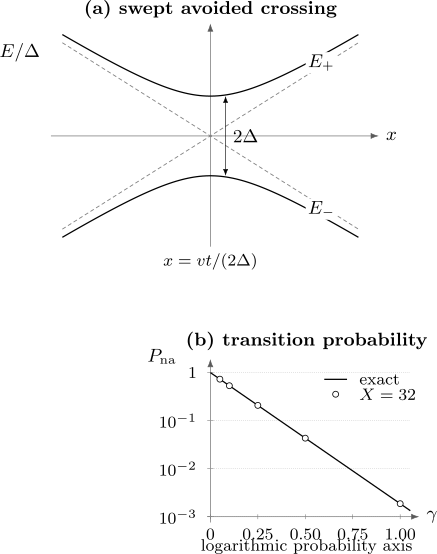
Dashed diabatic energies cross, while solid adiabatic energies retain a minimum gap $2\Delta$. In the lower panel the exact Landau–Zener law is a straight line on a logarithmic probability scale. Numerical points propagated on $-32\le x\le32$ lie on that line to the finite-window accuracy reported in the table.

Why Finite-Window Convergence Oscillates

The numerical values do not approach the asymptotic probability monotonically as $X$ increases. Far from the crossing, the residual moving-basis coupling is small but nonzero. Amplitude generated near an endpoint accumulates a rapidly varying dynamical phase before it interferes with the principal transition amplitude.

Consequently:

• increasing $X$ generally reduces the envelope of endpoint error;
• the signed error can change sign as the endpoint phase changes;
• agreement at one window is not a convergence study;
• halving the step at fixed $X$ tests integration error, not endpoint error.

A reliable numerical audit varies $h$ and $X$ separately. It also monitors norm preservation because explicit Runge–Kutta propagation is not exactly unitary.

The table’s $X=32$ discrepancy is therefore not evidence against the exact formula. Its scale and oscillatory sign are consistent with replacing asymptotic boundary conditions by finite endpoints.

What the Exact Formula Assumes

The exponential is exact for the ideal mathematical model, not for every experimental avoided crossing.

Isolated two-level subspace

Other levels must remain far enough away that their transition amplitudes are negligible. If several crossings overlap, a two-state reduction may fail even when each pairwise gap appears small.

Linear diabatic detuning

The energy difference must be well approximated by $vt$ over the transition region. A local Taylor expansion is useful only if quadratic and higher terms remain small during the interval that contributes appreciably to the transition amplitude.

Constant coupling

The off-diagonal matrix element is taken to be $\Delta$. A coupling that changes substantially through the crossing alters both the instantaneous gap and the transition law.

Infinite asymptotic preparation

The formula assumes well-defined incoming and outgoing states at $t\to\pm\infty$. Laboratory ramps and numerical calculations begin and end at finite detuning. Endpoint rotations and phases must be checked.

Coherent unitary dynamics

Relaxation, dephasing, noise, and measurement backaction are absent. Their importance is set by comparison of the crossing time and the relevant open-system timescales.

Single passage

Two or more coherent passages produce interference controlled by the dynamical phase accumulated between crossings and by the Landau–Zener scattering phase. Probabilities cannot generally be composed as classical independent events.

Validation Ledger

Check	Result
dimensions	$\Delta^2/(\hbar v)$ is dimensionless
zero coupling	$\Delta\to0$ gives $P_{\mathrm{na}}\to1$, meaning fixed diabatic character
slow sweep	$v\to0$ gives exponentially accurate adiabatic following
fast sweep	$v\to\infty$ gives the sudden diabatic limit
basis mapping	lower-branch following changes $\lvert1\rangle$ into $\lvert2\rangle$
complex-time action	reproduces the exact exponent
numerical propagation	agrees with the formula after independent $h$ and $X$ checks
norm	drift stays below $8.6\times10^{-9}$ in the reported calculation

Each check probes the ideal two-state calculation. None validates the omission of extra levels or environmental dynamics.

Common Mistakes

• Quoting $P_{\mathrm{LZ}}$ without identifying the Hamiltonian convention.
• Calling $e^{-2\pi\gamma}$ a diabatic transition probability when, in this setup, it is the probability to remain in the same diabatic state.
• Using $\Delta$ sometimes for the coupling and sometimes for the minimum gap without changing the exponent.
• Treating $v$ as the slope of one diagonal entry rather than the slope of their difference.
• Applying a local adiabatic inequality as though it were the exact final probability.
• Starting a finite-window propagation in a bare diabatic state and comparing directly with asymptotic adiabatic preparation.
• Checking step-size convergence while leaving the time window fixed and declaring the asymptotic answer verified.
• Ignoring norm drift in a nonunitary time-stepping scheme.
• Applying the single-passage formula to a coherent double passage without the Stückelberg phase.
• Using the closed two-level result when noise, relaxation, or nearby levels act on the crossing timescale.

Exercises

1. Track the basis labels

Show that lower-branch adiabatic following takes $\lvert1\rangle$ at $x\to-\infty$ into $\lvert2\rangle$ at $x\to+\infty$. What final state corresponds to the nonadiabatic probability?

Solution

As $x\to-\infty$, $\theta\to\pi$, so

$$\lvert-;x\rangle \longrightarrow -\lvert1\rangle.$$

As $x\to+\infty$, $\theta\to0$, so

$$\lvert-;x\rangle \longrightarrow \lvert2\rangle.$$

Following the lower adiabatic branch therefore transfers the diabatic population from $\lvert1\rangle$ to $\lvert2\rangle$. The nonadiabatic outcome ends on the upper branch, and

$$\lvert+;x\rangle \longrightarrow \lvert1\rangle$$

at positive infinity. Thus $P_{\mathrm{na}}$ is the same-diabatic-state probability for this preparation.

2. Derive the local adiabatic ratio

Starting from $\theta(x)=\operatorname{atan2}(1,x)$, derive $\mathcal A(x)$ and locate its maximum.

Solution

Differentiate:

$$\frac{d\theta}{dx} = - \frac{1}{1+x^2}.$$

Because

$$\frac{dx}{dt} = \frac{v}{2\Delta},$$

one finds

$$\lvert\dot\theta\rvert = \frac{ v }{ 2\Delta(1+x^2) }.$$

The off-diagonal derivative coupling has magnitude $\lvert\dot\theta\rvert/2$, while the gap is

$$G(t) = 2\Delta\sqrt{1+x^2}.$$

Therefore

$$\begin{aligned} \mathcal A(x) &= \frac{ \hbar v }{ 8\Delta^2 (1+x^2)^{3/2} } \\ &= \frac{ 1 }{ 8\gamma (1+x^2)^{3/2} }. \end{aligned}$$

The denominator is smallest at $x=0$, so $\mathcal A_{\max}=1/(8\gamma)$.

3. Design a sweep

Find the minimum $\gamma$ needed for $99.9\%$ adiabatic following. Express the corresponding maximum $v$ in terms of $\Delta$ and $\hbar$.

Solution

The allowed nonadiabatic error is

$$\varepsilon = 10^{-3}.$$

Thus

$$\gamma \ge \frac{ \ln(10^3) }{ 2\pi } \approx 1.099.$$

Since $\gamma=\Delta^2/(\hbar v)$,

$$v \le \frac{ 2\pi\Delta^2 }{ \hbar\ln(10^3) }.$$

This is the ideal infinite-sweep bound; a finite protocol needs additional endpoint and model-error margins.

4. Translate a convention

A paper uses

$$H(t) = \begin{pmatrix} \alpha t & g\\ g & -\alpha t \end{pmatrix}.$$

Write its nonadiabatic probability by identifying the diabatic slope and minimum gap.

Solution

The two diagonal entries differ by

$$2\alpha t,$$

so the slope corresponding to $v$ is $2\alpha$. The coupling corresponding to $\Delta$ is $g$, and the minimum gap is $2g$. Substitution into the convention used on this page gives

$$\begin{aligned} P_{\mathrm{na}} &= \exp\left[ - \frac{ 2\pi g^2 }{ \hbar(2\alpha) } \right] \\ &= \exp\left( - \frac{ \pi g^2 }{ \hbar\alpha } \right). \end{aligned}$$

5. Separate numerical errors

A calculation at fixed $X$ gives the same probability after halving $h$, but that value differs from the Landau–Zener formula. Name two possible explanations and a test for each.

Solution

First, the finite endpoints may not approximate $t\to\pm\infty$ accurately. Increase $X$ while continuing to resolve the larger endpoint frequencies. Because convergence can oscillate, compare several windows rather than only one.

Second, the initial or final basis may not match the asymptotic probability being tested. Prepare the exact instantaneous eigenstate at $-X$ and project onto the desired instantaneous eigenstate at $+X$.

If the discrepancy persists after both tests, inspect the propagated Hamiltonian, sign and factor conventions, norm drift, and whether the intended model actually has linear detuning and constant coupling.

Cross-Links

• Worked Problems and Model Calculations
• Landau–Zener Transition
• Landau–Zener Problem: First Encounter
• Adiabatic Approximation as a Method
• Sudden Approximation
• Two-State Hamiltonians
• Coupled Wells and Avoided Crossings
• Time-Dependent Hamiltonians
• Convergence Tests
• Landau–Zener Simulation

References

• L. D. Landau, “Zur Theorie der Energieübertragung. II,” Physikalische Zeitschrift der Sowjetunion 2, 46–51 (1932).
• C. Zener, “Non-Adiabatic Crossing of Energy Levels,” Proceedings of the Royal Society A 137, 696–702 (1932), doi:10.1098/rspa.1932.0165.
• E. C. G. Stückelberg, “Theorie der unelastischen Stösse zwischen Atomen,” Helvetica Physica Acta 5, 369–422 (1932).
• E. Majorana, “Atomi orientati in campo magnetico variabile,” Il Nuovo Cimento 9, 43–50 (1932), doi:10.1007/BF02960953.
• N. V. Vitanov and B. M. Garraway, “Landau–Zener model: Effects of finite coupling duration,” Physical Review A 53, 4288–4304 (1996), doi:10.1103/PhysRevA.53.4288.
• A. Joye, “Proof of the Landau–Zener Formula,” Asymptotic Analysis 9, 209–258 (1994).
• S. N. Shevchenko, S. Ashhab, and F. Nori, “Landau–Zener–Stückelberg interferometry,” Physics Reports 492, 1–30 (2010), doi:10.1016/j.physrep.2010.03.002.