Anharmonic Oscillator by Variational Methods

Consider the stable quartic oscillator

$$H = \frac{P^2}{2m} + \frac12m\omega^2X^2 + \lambda X^4, \qquad \lambda\geq0.$$

The goal is a one-parameter variational upper bound on its ground-state energy. The trial state will be a Gaussian with an adjustable frequency. Optimizing that frequency gives a compact approximation that agrees with weak-coupling perturbation theory at first order, remains meaningful when the perturbative truncation fails, and captures the correct strong-coupling power law.

This page owns the complete one-Gaussian calculation and its comparison with perturbative and numerical results. The Variational Principle owns the upper-bound theorem, Variational Parameters owns general optimization geometry, and Anharmonic Oscillator owns the model’s multi-method overview. The Variational Optimization Notebook extends this calculation to globally optimized finite Rayleigh-Ritz spaces and documents their numerical convergence.

Problem and Method Choice

For $\lambda>0$, the potential rises faster than a harmonic potential. Its ground state is therefore more localized than the ground state of the frequency-$\omega$ oscillator. A natural trial family is the set of harmonic-oscillator ground states with adjustable frequency $\Omega>0$.

This choice has four advantages:

• every trial state is normalized and has the correct even parity;
• $\Omega=\omega$ gives the exact ground state at $\lambda=0$;
• all required moments are analytic;
• increasing $\Omega$ narrows the state, allowing it to respond to the positive quartic confinement.

The method does not require the quartic coupling to be small for the upper-bound statement. Small coupling is needed only when the optimized result is expanded and compared order by order with ordinary perturbation theory. Accuracy at finite or strong coupling remains a property of the chosen Gaussian family and must be benchmarked.

Dimensionless Form

Introduce the harmonic length and dimensionless coordinate

$$b_0 = \sqrt{\frac{\hbar}{m\omega}}, \qquad q = \frac{X}{b_0},$$

and define

$$g = \frac{\lambda\hbar}{m^2\omega^3}.$$

Then the dimensionless Hamiltonian $h=H/(\hbar\omega)$ is

$$h = -\frac12\frac{d^2}{dq^2} + \frac12q^2 + gq^4.$$

All dependence on $m$, $\omega$, $\lambda$, and $\hbar$ has collapsed into the single nonnegative coupling $g$. The dimensional energy is recovered by multiplying by $\hbar\omega$.

Gaussian Trial Family

Use the normalized ground state of an oscillator with frequency $\Omega$:

$$\psi_\Omega(X) = \left( \frac{m\Omega}{\pi\hbar} \right)^{1/4} \exp\!\left( -\frac{m\Omega X^2}{2\hbar} \right).$$

It is convenient to optimize the frequency ratio

$$y = \frac{\Omega}{\omega} \gt0.$$

In the dimensionless coordinate,

$$\psi_y(q) = \left( \frac{y}{\pi} \right)^{1/4} e^{-yq^2/2}.$$

The corresponding width parameter is

$$x = \frac{b}{b_0} = y^{-1/2}.$$

Thus larger $y$ means a narrower state. Frequency and width parameterizations describe the same trial family; they should give the same physical minimum.

The Gaussian moments are

$$\langle q^2\rangle_y = \frac{1}{2y}, \qquad \langle q^4\rangle_y = \frac{3}{4y^2},$$

and, with $p_q=-i\,d/dq$,

$$\langle p_q^2\rangle_y = \frac{y}{2}.$$

These relations can be obtained from elementary Gaussian integrals or from ladder operators for the frequency-$y$ oscillator.

Rayleigh Quotient

The dimensionless energy expectation separates into kinetic, quadratic, and quartic pieces:

$$\begin{aligned} \varepsilon(y;g) \equiv{}& \langle\psi_y|h|\psi_y\rangle \\ ={}& \frac{y}{4} + \frac{1}{4y} + \frac{3g}{4y^2}. \end{aligned}$$

In dimensional variables, the same expression is

$$E(\Omega) = \frac{\hbar\Omega}{4} + \frac{\hbar\omega^2}{4\Omega} + \frac{3\lambda\hbar^2}{4m^2\Omega^2}.$$

Every term has energy units. The kinetic term penalizes excessive localization, while the quadratic and quartic potential terms penalize excessive spreading. Their competition produces a finite optimum.

Optimization

Stationarity gives

$$\frac{\partial\varepsilon}{\partial y} = \frac14 - \frac{1}{4y^2} - \frac{3g}{2y^3} = 0,$$

or equivalently

$$y_\star^3-y_\star-6g = 0.$$

For $g=0$, the physical root is $y_\star=1$, reproducing the exact harmonic ground state. For $g>0$, the left-hand side is negative at $y=1$ and strictly increasing for $y\geq1$. There is therefore one physical root with

$$y_\star>1.$$

The optimized Gaussian is narrower than the original oscillator ground state, as expected for an added positive quartic potential.

Using the stationary equation to eliminate $g$, the optimized energy simplifies to

$$\begin{aligned} \varepsilon_{\mathrm G}(g) ={}& \frac{3y_\star}{8} + \frac{1}{8y_\star} \\ ={}& \frac{3y_\star^2+1}{8y_\star}. \end{aligned}$$

The Rayleigh–Ritz theorem then gives the rigorous statement

$$E_0(g) \leq E_{\mathrm G}(g) = \hbar\omega\, \varepsilon_{\mathrm G}(g)$$

for every $g\geq0$.

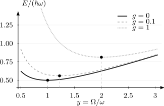
The Rayleigh quotient diverges when the Gaussian is made too broad and rises again when it is made too narrow. Positive quartic coupling moves the minimum to $y_\star>1$, corresponding to a narrower position-space state. Each marked minimum is an upper bound on the exact ground energy at that coupling.

Weak-Coupling Comparison

For $g\ll1$, solve the cubic perturbatively:

$$y_\star = 1 + 3g - \frac{27}{2}g^2 + O(g^3).$$

Substitution into the optimized energy gives

$$\varepsilon_{\mathrm G}(g) = \frac12 + \frac34g - \frac94g^2 + O(g^3).$$

Ordinary Rayleigh–Schrödinger perturbation theory gives

$$\varepsilon_0(g) = \frac12 + \frac34g - \frac{21}{8}g^2 + O(g^3).$$

The complete coefficient derivation is in Anharmonic Oscillator by Perturbation Theory. Comparing the two expansions,

$$\varepsilon_{\mathrm G}(g) - \varepsilon_0(g) = \frac38g^2 + O(g^3).$$

The Gaussian result reproduces the exact first-order coefficient. This is not an accident. At $g=0$ the trial family contains the exact state, and the unperturbed energy is stationary with respect to $y$. The $O(g)$ shift of the optimum therefore does not change the harmonic contribution at first order; only the explicit expectation of $gq^4$ contributes.

At second order, the exact state develops components that cannot be represented by changing one Gaussian width. The positive difference is consistent with the variational upper bound.

There is an important logical distinction: the fully minimized $\varepsilon_{\mathrm G}(g)$ is an upper bound, but a finite Taylor truncation of that function need not remain an upper bound at arbitrary $g$.

Strong-Coupling Limit

When $g\gg1$, the cubic gives

$$y_\star \sim (6g)^{1/3},$$

so the optimal width scales as

$$x_\star = y_\star^{-1/2} \sim (6g)^{-1/6}.$$

The energy becomes

$$\varepsilon_{\mathrm G}(g) \sim \frac38(6g)^{1/3}.$$

Thus the Gaussian captures the exact quartic-oscillator scaling $E_0\propto g^{1/3}$. Its leading coefficient is

$$\frac38,6^{1/3} \approx 0.68142.$$

Converged numerical diagonalization of the pure quartic Hamiltonian gives approximately

$$\varepsilon_0(g) \sim 0.667986\,g^{1/3}.$$

The one-Gaussian coefficient is about two percent high, as an upper bound should be. The correct scaling follows from balancing kinetic and quartic energies; the remaining coefficient error measures the limited shape of the ansatz.

Numerical Benchmark

An independent benchmark expands

$$h = \left(a^\dagger a+\frac12\right) + gq^4$$

in the frequency-one oscillator basis and diagonalizes a truncated matrix. Because parity is exact, the even sector can be treated separately. The basis size must be increased until the low eigenvalue is stable.

The following values use a converged oscillator-basis diagonalization. Energies are in units of $\hbar\omega$.

$g$	$y_\star$	Numerical $E_0$	Gaussian Bound	Relative Excess
$0.01$	$1.028748$	$0.507256$	$0.507288$	$0.0062\%$
$0.10$	$1.221197$	$0.559146$	$0.560307$	$0.208\%$
$1$	$2$	$0.803771$	$0.812500$	$1.09\%$
$10$	$4$	$1.504972$	$1.531250$	$1.75\%$

The same comparison exposes the limited range of low-order perturbation theory:

$g$	Numerical $E_0$	First Order	Through Second Order
$0.01$	$0.507256$	$0.507500$	$0.507238$
$0.10$	$0.559146$	$0.575000$	$0.548750$
$1$	$0.803771$	$1.250000$	$-1.375000$

At weak coupling, perturbation theory resolves the local series more systematically. At moderate and strong coupling, its low-order polynomial truncations lose usefulness, while the optimized Gaussian remains positive, variational, and correctly scaled. This does not make the Gaussian uniformly more accurate than all perturbative reorganizations; it shows that the two methods encode different information.

Perturbation Theory Benchmarks owns the numerical convergence workflow and broader parameter sweeps.

Virial and Residual Checks

Optimization with respect to a scale parameter enforces a virial identity. For the dimensionless potential

$$V(q) = \frac12q^2+gq^4,$$

the exact virial theorem is

$$2\langle T\rangle = \langle q^2\rangle + 4g\langle q^4\rangle.$$

In the optimized Gaussian this becomes

$$\frac{y_\star}{2} = \frac{1}{2y_\star} + \frac{3g}{y_\star^2},$$

which is precisely the stationary cubic after multiplication by $2y_\star^2$. The variational state therefore satisfies the virial relation exactly even though it is not an exact eigenstate.

The eigenstate residual reveals what remains missing. Let $|n_y\rangle$ denote oscillator states of frequency ratio $y$. Acting on the optimized trial state gives

$$\left( h-\varepsilon_{\mathrm G} \right) |0_{y_\star}\rangle = \frac{\sqrt6\,g}{2y_\star^2} |4_{y_\star}\rangle.$$

The $|2_y\rangle$ component vanishes because the width has been optimized. The surviving $|4_y\rangle$ component cannot be removed by moving along the one-parameter Gaussian family. Consequently,

$$\left| \left( h-\varepsilon_{\mathrm G} \right) |0_{y_\star}\rangle \right|^2 = \frac{3g^2}{2y_\star^4}.$$

This residual is a state-quality diagnostic, not an additional variational bound. It suggests the next improvement: enlarge the trial space with non-Gaussian even components, or use Rayleigh–Ritz diagonalization in several $|n_y\rangle$ states.

Result and Validity

The calculation can be summarized without solving the cubic in radicals:

$$\begin{gathered} y_\star^3-y_\star-6g=0, \\ y_\star\geq1, \\ \frac{E_{\mathrm G}}{\hbar\omega} = \frac{3y_\star^2+1}{8y_\star}, \\ E_0\leq E_{\mathrm G}. \end{gathered}$$

The upper bound is rigorous for the stated Hamiltonian and every $g\geq0$. Its numerical accuracy is not rigorous without further spectral information. The benchmark indicates that this particular one-Gaussian energy is accurate from weak coupling through the pure-quartic regime at roughly the percent level or better, but wavefunction-sensitive observables can have larger errors.

The calculation does not apply unchanged to $g<0$. The potential is then unbounded below, and the relevant physics concerns metastability and resonances rather than a normalizable ground state. Excited-state estimates also require orthogonality constraints or the min–max principle; minimizing an unconstrained Gaussian always targets the ground state.

Common Mistakes

• Forgetting to normalize the Gaussian before evaluating moments.
• Treating $\Omega$ as a new physical frequency rather than a variational parameter.
• Choosing a stationary root without checking $y>0$ and the global minimum.
• Claiming that the positive quartic term broadens the ground state; for $g>0$, it gives $y_\star>1$ and narrows the Gaussian.
• Calling the difference between two variational estimates an exact error bar.
• Assuming a good variational energy guarantees accurate tails or higher moments.
• Treating the Taylor expansion of the optimized bound as a bound at finite coupling.
• Applying the ground-state inequality to a metastable negative-coupling problem.

Exercises

1. Derive the Gaussian moments

Starting from $\psi_y(q)$, derive $\langle q^2\rangle_y$, $\langle q^4\rangle_y$, and $\langle p_q^2\rangle_y$.

Solution

The probability density is

$$|\psi_y(q)|^2 = \sqrt{\frac{y}{\pi}}e^{-yq^2}.$$

Standard Gaussian moments give

$$\langle q^2\rangle_y = \frac{1}{2y}, \qquad \langle q^4\rangle_y = 3\langle q^2\rangle_y^2 = \frac{3}{4y^2}.$$

Because $d\psi_y/dq=-yq\psi_y$,

$$\langle p_q^2\rangle_y = \int dq\, \left| \frac{d\psi_y}{dq} \right|^2 = y^2\langle q^2\rangle_y = \frac{y}{2}.$$

2. A coupling with an exact trial-frequency root

Show that $g=1$ has $y_\star=2$, and compute the Gaussian bound. Compare it with the numerical value in the table.

Solution

The stationary equation is $y^3-y-6g=0$. At $g=1$,

$$2^3-2-6=0,$$

so $y_\star=2$. The optimized energy is

$$\begin{aligned} \varepsilon_{\mathrm G} ={}& \frac{3(2)}{8} + \frac{1}{8(2)} \\ ={}& \frac{13}{16} = 0.8125. \end{aligned}$$

Compared with $E_0\approx0.803771$, the relative excess is about $1.09\%$.

3. Expand the optimized energy

Derive $y_\star=1+3g-27g^2/2+O(g^3)$ and use it to obtain the Gaussian energy through $O(g^2)$.

Solution

Write $y_\star=1+ag+bg^2+O(g^3)$. Expanding $y^3-y-6g=0$ gives

$$(2a-6)g + (3a^2+2b)g^2 + O(g^3) = 0.$$

Hence $a=3$ and $b=-27/2$. Substituting into

$$\varepsilon_{\mathrm G} = \frac{3y_\star}{8} + \frac{1}{8y_\star}$$

gives

$$\varepsilon_{\mathrm G} = \frac12 + \frac34g - \frac94g^2 + O(g^3).$$

4. Verify the residual

Using

$$q = \frac{a_y+a_y^\dagger}{\sqrt{2y}},$$

show that optimization cancels the $|2_y\rangle$ part of $(h-\varepsilon)|0_y\rangle$ and leaves the stated $|4_y\rangle$ residual.

Solution

The required actions are

$$q^2|0_y\rangle = \frac{1}{2y} \left( |0_y\rangle + \sqrt2|2_y\rangle \right),$$

and

$$\begin{aligned} q^4|0_y\rangle ={}& \frac{1}{4y^2} \left( 3|0_y\rangle + 6\sqrt2|2_y\rangle \right. \\ &\left. + 2\sqrt6|4_y\rangle \right). \end{aligned}$$

Write

$$h = h_y + \frac12(1-y^2)q^2 + gq^4,$$

where $h_y|0_y\rangle=(y/2)|0_y\rangle$. The $|2_y\rangle$ coefficient is proportional to

$$y-y^3+6g,$$

which vanishes at the stationary point. Subtracting the expectation value removes the $|0_y\rangle$ component. The remaining term is

$$\frac{\sqrt6\,g}{2y^2}|4_y\rangle.$$

5. Recover the strong-coupling scaling

Use a length-balance argument, without the stationary cubic, to derive the powers $x_\star\propto g^{-1/6}$ and $E\propto g^{1/3}$.

Solution

For a state of dimensionless width $x$, kinetic energy scales as $x^{-2}$ and quartic energy as $gx^4$. Balancing the two contributions gives

$$x^{-2} \sim gx^4,$$

so $x^6\sim g^{-1}$ and

$$x\sim g^{-1/6}.$$

Either balanced energy then scales as

$$x^{-2} \sim g^{1/3}.$$

The variational calculation fixes the numerical coefficient within the Gaussian family.

Cross-Links

• Worked Problems and Model Calculations
• Anharmonic Oscillator by Perturbation Theory
• Anharmonic Oscillator
• Variational Principle
• Trial Wavefunctions
• Variational Parameters
• Gaussian Variational Methods
• Variational Perturbation Theory
• Variational Optimization Notebook
• Perturbation Theory Benchmarks
• Matrix Diagonalization

References

• R. Shankar, Principles of Quantum Mechanics, 2nd ed., Springer, 1994.
• J. J. Sakurai and J. Napolitano, Modern Quantum Mechanics, 3rd ed., Cambridge University Press, 2020.
• C. M. Bender and T. T. Wu, “Anharmonic oscillator,” Physical Review 184, 1231–1260, 1969.
• C. M. Bender and T. T. Wu, “Anharmonic oscillator. II. A study of perturbation theory in large order,” Physical Review D 7, 1620–1636, 1973.
• C. M. Bender and S. A. Orszag, Advanced Mathematical Methods for Scientists and Engineers, Springer, 1999.
• B. Simon, “Coupling constant analyticity for the anharmonic oscillator,” Annals of Physics 58, 76–136, 1970.