Variational Parameters

A variational parameter is a coordinate on a chosen family of trial states. Widths, orbital exponents, mixing angles, correlation lengths, tensor entries, and circuit rotations all play this role. Optimizing them means finding the lowest Rayleigh quotient accessible to that family, not solving the unrestricted Hilbert-space problem.

This page is the canonical home for parameter optimization. It derives energy gradients, explains tangent-space stationarity, distinguishes ordinary and geometry-aware updates, analyzes Hessians and constraints, and gives numerical diagnostics. The Variational Principle owns the upper-bound proof, while Trial Wavefunctions owns the physical design of the ansatz.

Parameterized Rayleigh Quotient

Let

$$\boldsymbol\theta = (\theta^1,\ldots,\theta^p) \in \mathcal P$$

be real parameters and let $\lvert\psi(\boldsymbol\theta)\rangle$ be a differentiable family of nonzero admissible states. For a fixed Hamiltonian $H$, define

$$E(\boldsymbol\theta) = \frac{ \langle\psi(\boldsymbol\theta)\rvert H \lvert\psi(\boldsymbol\theta)\rangle }{ \langle\psi(\boldsymbol\theta) \vert \psi(\boldsymbol\theta)\rangle }.$$

The parameter optimum is

$$E_{\mathrm{opt}} = \inf_{\boldsymbol\theta\in\mathcal P} E(\boldsymbol\theta).$$

The distinction between minimum and infimum matters. A parameter can run toward a boundary or infinity while the energy approaches a limiting value that is never attained inside $\mathcal P$. Compact parameter ranges do not arise automatically.

Three spaces should remain conceptually separate:

1. Parameter space $\mathcal P$, where the optimizer moves.
2. Trial manifold $\mathcal M$, the set of physical rays represented by the ansatz.
3. Hilbert space, which contains both $\mathcal M$ and states the ansatz cannot represent.

Different parameter values can represent the same physical ray. Overall phase, normalization, periodic angles, tensor-network gauge transformations, and redundant basis functions all create such nonuniqueness.

Derivative of the Energy

Write

$$N(\boldsymbol\theta) = \langle\psi\vert\psi\rangle, \qquad \lvert\partial_a\psi\rangle = \frac{\partial}{\partial\theta^a} \lvert\psi\rangle.$$

For fixed $H$, quotient differentiation gives

$$\begin{aligned} \partial_a E ={}& \frac{ \langle\partial_a\psi\rvert H\lvert\psi\rangle + \langle\psi\rvert H\lvert\partial_a\psi\rangle }{N} \\ &- E \frac{ \langle\partial_a\psi\vert\psi\rangle + \langle\psi\vert\partial_a\psi\rangle }{N}. \end{aligned}$$

Introduce the residual

$$\lvert r\rangle = (H-E)\lvert\psi\rangle.$$

Then the gradient component has the compact form

$$\partial_a E = \frac{2}{N} \operatorname{Re} \langle\partial_a\psi\vert r\rangle.$$

This formula is valid whether or not the ansatz is explicitly normalized. It also reveals the central geometry: at a stationary point, the residual is real-orthogonal to every parameter tangent,

$$\operatorname{Re} \langle\partial_a\psi\vert r\rangle = 0, \qquad a=1,\ldots,p.$$

The residual need not vanish. Optimization only removes its components visible inside the tangent space of the trial family.

Normalized states

If $N=1$ for every parameter value, differentiation of the normalization condition gives

$$2\operatorname{Re} \langle\psi\vert\partial_a\psi\rangle = 0.$$

The tangent can still contain a purely imaginary component parallel to $\lvert\psi\rangle$, corresponding to a parameter-dependent phase. Because

$$\langle\psi\vert r\rangle = 0,$$

that phase direction does not affect the energy gradient.

Complex parameters

For complex parameters, either split each one into real and imaginary parts or use Wirtinger derivatives with $z^a$ and $z^{a*}$ treated as independent coordinates. The stationarity conditions must include both real directions. Differentiating only with respect to $z^a$ can miss half of the optimization problem unless the analytic structure is stated carefully.

Tangent Vectors and the State-Space Metric

Normalized vectors that differ only by overall phase represent the same physical state. Remove the phase-and-normalization component of a parameter derivative by defining

$$\lvert D_a\psi\rangle = \left( I- \lvert\psi\rangle\langle\psi\rvert \right) \lvert\partial_a\psi\rangle.$$

For normalized states,

$$\partial_a E = 2\operatorname{Re} \langle D_a\psi\vert r\rangle.$$

The real part of the pulled-back quantum geometric tensor defines a metric on nonredundant parameter directions:

$$G_{ab} = \operatorname{Re} \langle D_a\psi\vert D_b\psi\rangle.$$

Equivalently,

$$\begin{aligned} G_{ab} ={}& \operatorname{Re} \bigl[ \langle\partial_a\psi \vert\partial_b\psi\rangle \\ &- \langle\partial_a\psi\vert\psi\rangle \langle\psi\vert\partial_b\psi\rangle \bigr]. \end{aligned}$$

This metric measures how much the physical state changes, rather than how far the raw coordinates move. It is positive semidefinite. A zero eigenvalue identifies a locally redundant parameter combination, although nearly zero eigenvalues can also arise from weak sensitivity over the sampled region.

The full geometric interpretation belongs to Fubini–Study Geometry. For optimization, the practical lesson is immediate: equal Euclidean steps in two parameters need not produce equal changes in the state.

Geometry-aware updates

Let

$$g_a = \partial_a E.$$

An ordinary gradient step is

$$\delta\theta^a = -\eta g_a.$$

A metric-scaled or natural-gradient step solves

$$\sum_b \left( G_{ab}+\lambda\delta_{ab} \right) \delta\theta^b = -\eta g_a,$$

where $\lambda\geq0$ is a damping parameter. With a pseudoinverse, this suppresses null directions and rescales directions according to the state-space geometry.

Natural-gradient language does not create a universal optimizer. The metric can be noisy, singular, expensive to form, or only locally informative. Damping, trust regions, and independent convergence checks remain necessary.

Multiple Parameters and Stationarity

For an unconstrained interior optimum $\boldsymbol\theta_\star$,

$$\nabla_{\boldsymbol\theta}E \big|_{\boldsymbol\theta_\star} = 0.$$

This condition is necessary, not sufficient. It can describe a local minimum, maximum, saddle, or flat manifold of equivalent parameterizations.

Coordinate dependence of gradients

Suppose $\boldsymbol\eta$ is another smooth coordinate system with

$$\theta^a = \theta^a(\boldsymbol\eta).$$

The gradient components transform by the chain rule:

$$\frac{\partial E}{\partial\eta^i} = \sum_a \frac{\partial\theta^a}{\partial\eta^i} \frac{\partial E}{\partial\theta^a}.$$

The statement that the gradient vanishes is coordinate independent at a nonsingular change of variables. The numerical size of the gradient is not. A stopping rule such as $\lVert\nabla E\rVert\lt\varepsilon$ is meaningless until the parameter scaling and norm have been specified.

Linear coefficients as variational parameters

For

$$\lvert\psi\rangle = \sum_j c_j\lvert\phi_j\rangle,$$

stationarity with respect to all real and imaginary coefficient directions gives

$$Hc=ESc.$$

Thus the generalized eigenvalue equation is the exact coefficient-stationarity condition inside a linear trial space. Nonlinear parameters in the basis functions require an additional outer optimization. See the Rayleigh–Ritz Method.

Constraints and Reparameterization

Constraints are often best enforced by construction. An optimizer should not be allowed to step outside the domain where the trial state is meaningful.

Positive parameters

If a width $b$ must satisfy $b\gt0$, write

$$b = b_{\mathrm{ref}}e^\eta, \qquad \eta\in\mathbb R.$$

Then

$$\frac{dE}{d\eta} = b\frac{dE}{db}.$$

At a stationary point,

$$\frac{d^2E}{d\eta^2} = b^2\frac{d^2E}{db^2},$$

because the term $b,dE/db$ vanishes there. Logarithmic coordinates enforce positivity and make multiplicative scale changes additive.

Normalization

Explicit normalization can be built into the ansatz, or the Rayleigh quotient can remove a free overall scale. Treating normalization as an independent unconstrained parameter creates a flat direction. If one instead minimizes $\langle\psi\rvert H\lvert\psi\rangle$ subject to $\langle\psi\vert\psi\rangle=1$, a Lagrange multiplier produces the eigenvalue equation.

Equality constraints

For constraints

$$C_\mu(\boldsymbol\theta) = 0, \qquad \mu=1,\ldots,q,$$

the first-order condition is

$$\nabla E + J_C^{\mathsf T} \boldsymbol\lambda = 0,$$

where

$$(J_C)_{\mu a} = \frac{\partial C_\mu}{\partial\theta^a}.$$

Equivalently, the gradient must vanish along every tangent direction that preserves the constraints to first order.

Symmetry constraints

Particle exchange, parity, angular momentum, gauge constraints, and boundary conditions should usually be built into the state family rather than imposed through a large energy penalty. A finite penalty changes the objective and can leave symmetry contamination. Projection methods can restore a symmetry, but their normalization and parameter derivatives must then be included consistently.

Hessians and Local Curvature

The parameter Hessian is

$$K_{ab} = \frac{\partial^2E}{ \partial\theta^a\partial\theta^b }.$$

At an unconstrained local minimum, $K$ is positive semidefinite. It is positive definite only after redundant directions and continuous degeneracies have been removed. A negative eigenvalue identifies a descent direction, while a zero eigenvalue can signal symmetry, gauge redundancy, an underdetermined ansatz, or a higher-order flat direction.

Curvature at an exact eigenstate

Suppose a normalized ansatz passes through an exact eigenstate $\lvert n\rangle$ at $\boldsymbol\theta_0$. Since the residual vanishes there, the Hessian simplifies to

$$K_{ab} = 2\operatorname{Re} \langle D_a n\rvert (H-E_n) \lvert D_b n\rangle.$$

For the ground state, this quadratic form is nonnegative. For an excited eigenstate, tangent directions that overlap lower-energy states produce negative curvature unless symmetry or orthogonality constraints exclude them. An excited eigenstate is therefore typically a saddle of the unrestricted energy functional. Rigorous excited-state bounds use the ordered subspace construction developed in Upper Bounds and the Min–Max Principle.

Stiff and soft directions

Let the nonzero Hessian eigenvalues near a minimum be

$$0\lt\kappa_{\min} \leq \kappa_i \leq \kappa_{\max}.$$

The ratio

$$\operatorname{cond}(K) = \frac{\kappa_{\max}}{\kappa_{\min}}$$

measures local anisotropy in the chosen coordinates. A large ratio creates a narrow valley: steps stable in the stiff direction make painfully slow progress along the soft direction. This is an optimization-conditioning problem, not automatically evidence of a poor ansatz.

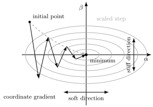
Elongated contours indicate very different curvatures along two parameter combinations. Unscaled coordinate-gradient steps can zigzag across a stiff direction; curvature or state-metric information can propose a better-scaled local step. Neither path changes the trial family’s ansatz error.

The numerical interpretation of condition numbers and stability is developed in Conditioning and Stability.

Scale Analysis Before Optimization

Physical dimensions should be removed before handing a problem to a numerical optimizer. If one parameter is measured in inverse ångströms and another in joules, an ordinary Euclidean gradient combines incomparable coordinate components.

A useful workflow is:

1. identify natural length, energy, and time scales from the Hamiltonian;
2. express the ansatz in dimensionless variables;
3. center parameters near physically plausible values;
4. use logarithmic variables for positive scales spanning orders of magnitude;
5. inspect Hessian or metric eigenvalues after the transformation.

Good scaling does not alter the physical trial family. It changes the chart used to search it.

Scale Translation: Quartic Gaussian Width

The quartic oscillator provides a compact example of why scaling should precede optimization. With

$$x = \frac{b}{\sqrt{\hbar/(m\omega)}}, \qquad \gamma = \frac{\lambda\hbar}{m^2\omega^3},$$

the Gaussian Rayleigh quotient becomes

$$\frac{E(x)}{\hbar\omega} = \frac{1}{4x^2} + \frac{x^2}{4} + \frac{3\gamma x^4}{4}.$$

The positive parameter $x$ is dimensionless and order unity at weak coupling. Frequency notation uses $y=\Omega/\omega=x^{-2}$, so the same stationary condition can be written in either chart:

$$-1+x^4+6\gamma x^6=0 \quad\Longleftrightarrow\quad y^3-y-6\gamma=0.$$

The complete normalization, minimization, weak- and strong-coupling limits, upper-bound interpretation, residual analysis, and numerical comparison belong to Anharmonic Oscillator by Variational Methods. The coordinate lesson needed here is that the physical optimum is unchanged by the smooth reparameterization $y=x^{-2}$, while gradients and curvatures acquire different numerical scales.

Parameter-Dependent Bases

Suppose a nonorthogonal basis depends on a nonlinear parameter $\alpha$ and the optimized coefficients solve

$$H(\alpha)c = E(\alpha)S(\alpha)c,$$

with normalization

$$c^\dagger S c = 1.$$

At an exactly solved generalized eigenpair,

$$\frac{dE}{d\alpha} = c^\dagger \left( \frac{dH}{d\alpha} - E\frac{dS}{d\alpha} \right) c.$$

The $dS/d\alpha$ term is essential. It records the changing basis geometry and is a finite-dimensional relative of a Pulay term. Ignoring it treats a moving nonorthogonal basis as fixed and generally gives the wrong gradient.

If the coefficient eigenproblem is not converged, additional response terms survive. The clean derivative formula relies on stationarity with respect to $c$.

Optimized Energies and the Envelope Principle

Let the Hamiltonian depend on a physical control parameter $\lambda$, and define

$$E_\star(\lambda) = E( \boldsymbol\theta_\star(\lambda), \lambda ).$$

The total derivative is

$$\frac{dE_\star}{d\lambda} = \left. \frac{\partial E}{\partial\lambda} \right|_{\boldsymbol\theta} + \sum_a \frac{\partial E}{\partial\theta^a} \frac{d\theta^a_\star}{d\lambda}.$$

At an unconstrained stationary optimum, the second term vanishes:

$$\frac{dE_\star}{d\lambda} = \left. \frac{\partial E}{\partial\lambda} \right|_{\boldsymbol\theta_\star}.$$

This is why optimized variational energies often have simple first derivatives even though the optimal parameters move. Incomplete optimization, changing constraints, and parameter-dependent bases can restore response terms. The operator-derivative statement and its caveats are treated in the Hellmann–Feynman Theorem.

Choosing a Numerical Optimizer

No optimizer repairs a trial family that cannot represent the needed physics. Within a reasonable family, the method should match the parameter count, smoothness, conditioning, constraints, and noise level.

Method	Useful when	Main caution
Analytic stationarity	One or a few parameters and tractable integrals	Roots can be maxima or saddles
Gradient descent with line search	Gradients are reliable and scaling is moderate	Slow in narrow valleys
Conjugate-gradient or quasi-Newton	Smooth medium-to-large problems	Curvature models can be corrupted by noise
Newton or trust-region method	Accurate Hessian information is affordable	Hessians can be indefinite or singular
Derivative-free search	Very few parameters or nonsmooth evaluations	Scales poorly with dimension
Natural gradient or stochastic reconfiguration	State geometry is important or Monte Carlo samples provide the metric	Metric estimation, damping, and rank control are delicate

Line searches and trust regions

A descent direction is not enough. A line search chooses a step length that actually lowers the objective, while a trust region limits the update to a neighborhood where the local model is credible. In noisy calculations, requiring a decrease much smaller than the estimator uncertainty has no statistical meaning.

Stochastic objectives

In variational Monte Carlo, the energy, gradient, and metric are sample estimates. Reusing correlated samples can reduce the noise in energy differences, but it also complicates uncertainty estimates. Optimization bias and final statistical uncertainty should be assessed with fresh samples. See Variational Monte Carlo Preview.

Automatic differentiation

Automatic differentiation can evaluate exact derivatives of the implemented computational graph. It does not certify that the graph represents the intended Hamiltonian, normalization, boundary conditions, or sampling distribution. Analytic limits and finite-difference spot checks remain valuable.

Verification Checklist

Before accepting optimized parameters, record the following.

1. Admissibility: every iterate used for the final result defines a normalizable state with finite energy and correct symmetry.
2. Independent gradient check: compare analytic or automatic derivatives with finite differences at several points and step sizes.
3. Multiple starts: rerun from physically distinct initial points when local minima are possible.
4. Stationarity: report a scaled gradient norm or projected residual, not only the final energy change.
5. Curvature: inspect Hessian or metric eigenvalues for negative, zero, and poorly determined directions.
6. Stability: vary damping, trust radius, integration tolerance, basis threshold, or sample size.
7. State diagnostics: check the residual, energy variance, symmetry, and scientifically relevant observables.
8. Ansatz comparison: compare independent trial families or systematically enlarged spaces.
9. Uncertainty: separate optimizer tolerance, deterministic numerical error, and stochastic error.

Common Mistakes

• Varying a parameter that only rescales or rephases the state and then interpreting the resulting flat direction as physics.
• Declaring convergence because successive energies agree while the gradient remains large in a poorly scaled direction.
• Using $\partial_a\langle\psi\rvert H\lvert\psi\rangle$ as the gradient while forgetting the normalization derivative.
• Treating every stationary point as a minimum.
• Comparing raw gradient components with incompatible units.
• Allowing a positive width, decay constant, or covariance eigenvalue to cross into an invalid region.
• Ignoring $dS/d\alpha$ when nonlinear parameters move a nonorthogonal basis.
• Inverting a nearly singular Hessian or state metric without rank control or damping.
• Reporting a stochastic energy decrease smaller than its correlated uncertainty.
• Assuming that a perfectly optimized ansatz has no ansatz error.

The chapter’s Common Variational Pitfalls guide shows how these optimizer symptoms differ from domain, symmetry, expressivity, and interpretation failures.

Exercises

1. Derive the Rayleigh-quotient gradient

Starting from

$$E = \frac{\langle\psi\rvert H\lvert\psi\rangle}{ \langle\psi\vert\psi\rangle },$$

derive

$$\partial_aE = \frac{2}{N} \operatorname{Re} \langle\partial_a\psi\vert(H-E)\lvert\psi\rangle.$$

Solution

Let

$$A = \langle\psi\rvert H\lvert\psi\rangle, \qquad N = \langle\psi\vert\psi\rangle.$$

Then

$$\partial_aE = \frac{N\partial_aA-A\partial_aN}{N^2}.$$

For fixed Hermitian $H$,

$$\partial_aA = 2\operatorname{Re} \langle\partial_a\psi\rvert H\lvert\psi\rangle,$$ $$\partial_aN = 2\operatorname{Re} \langle\partial_a\psi\vert\psi\rangle.$$

Using $A=EN$ gives

$$\partial_aE = \frac{2}{N} \operatorname{Re} \langle\partial_a\psi\rvert(H-E)\lvert\psi\rangle.$$

2. Recover Rayleigh–Ritz stationarity

Let $\lvert\psi\rangle=\sum_jc_j\lvert\phi_j\rangle$ in a nonorthogonal basis. Vary the real and imaginary parts of $c_j$ and show that stationarity of the Rayleigh quotient gives $Hc=ESc$.

Solution

The quotient is

$$E(c) = \frac{c^\dagger Hc}{c^\dagger Sc}.$$

Treating $c$ and $c^*$ as independent Wirtinger variables,

$$\frac{\partial E}{\partial c^*} = \frac{ Hc(c^\dagger Sc) - Sc(c^\dagger Hc) }{ (c^\dagger Sc)^2 }.$$

Since $c^\dagger Hc=E,c^\dagger Sc$, stationarity gives

$$Hc-ESc = 0.$$

Variations of $c$ give the Hermitian-conjugate equation.

3. Logarithmic width coordinate

Let $b=b_{\mathrm{ref}}e^\eta$. Derive the first and second derivatives of $E$ with respect to $\eta$, and simplify the second derivative at a stationary point in $b$.

Solution

Because $db/d\eta=b$,

$$\frac{dE}{d\eta} = b\frac{dE}{db}.$$

Differentiating again,

$$\frac{d^2E}{d\eta^2} = b\frac{dE}{db} + b^2\frac{d^2E}{db^2}.$$

At $dE/db=0$,

$$\left. \frac{d^2E}{d\eta^2} \right|_\star = b_\star^2 \left. \frac{d^2E}{db^2} \right|_\star.$$

Thus the sign of the curvature at an interior stationary point is unchanged, while its numerical scale changes.

4. Translate width and frequency coordinates

For the quartic Gaussian example, let $y=x^{-2}$. Show that

$$-1+x^4+6\gamma x^6=0$$

is equivalent to $y^3-y-6\gamma=0$. Which direction does the optimum move for $\gamma>0$?

Solution

Substituting $x^2=y^{-1}$ and multiplying the width equation by $y^3$ gives

$$-y^3+y+6\gamma=0,$$

or

$$y^3-y-6\gamma=0.$$

For $\gamma>0$, the physical root has $y>1$. Therefore $x=y^{-1/2}<1$: the optimized frequency increases while the position-space width decreases. The full calculation is in Anharmonic Oscillator by Variational Methods.

5. Why an excited eigenstate is a saddle

Consider a normalized path through $\lvert n\rangle$ with tangent component along a lower eigenstate $\lvert m\rangle$, where $E_m\lt E_n$. Use the exact-eigenstate Hessian to determine the sign of the curvature along that direction.

Solution

Take a projected tangent $\lvert D\psi\rangle=a\lvert m\rangle$. The second variation is proportional to

$$\begin{gathered} 2\langle D\psi\rvert (H-E_n) \lvert D\psi\rangle \\ = 2\lvert a\rvert^2 (E_m-E_n) \\ \lt0. \end{gathered}$$

Since $E_m-E_n\lt0$, the curvature is negative. The energy decreases by mixing in the lower state, so the excited eigenstate is not a local minimum in the unrestricted state space. A symmetry or orthogonality constraint can remove this direction.

6. Derivative in a moving nonorthogonal basis

Differentiate $Hc=ESc$ with respect to $\alpha$, left-multiply by $c^\dagger$, and use $c^\dagger H=E c^\dagger S$ and $c^\dagger Sc=1$ to derive the parameter-dependent-basis formula.

Solution

Differentiation gives

$$H'c+Hc' = E'Sc+ES'c+ESc'.$$

Left-multiplying by $c^\dagger$ yields

$$\begin{aligned} c^\dagger H'c + c^\dagger Hc' ={}& E'c^\dagger Sc \\ &+ E c^\dagger S'c + E c^\dagger Sc'. \end{aligned}$$

Using $c^\dagger H=E c^\dagger S$ cancels the terms containing $c'$, and $c^\dagger Sc=1$ gives

$$E' = c^\dagger(H'-ES')c.$$

The overlap derivative cannot be discarded when the basis moves.

References

1. J. Nocedal and S. J. Wright, Numerical Optimization, 2nd ed. (Springer, 2006). Standard reference for line searches, trust regions, quasi-Newton methods, constraints, and conditioning.
2. S.-i. Amari, “Natural Gradient Works Efficiently in Learning”, Neural Computation 10, 251–276 (1998). Foundational account of metric-aware parameter optimization.
3. C. J. Umrigar, K. G. Wilson, and J. W. Wilkins, “Optimized Trial Wave Functions for Quantum Monte Carlo Calculations”, Physical Review Letters 60, 1719–1722 (1988). Classic treatment of trial-state optimization in variational Monte Carlo.
4. S. Sorella, “Green Function Monte Carlo with Stochastic Reconfiguration”, Physical Review Letters 80, 4558–4561 (1998). Introduces stochastic reconfiguration in a many-body Monte Carlo setting.
5. J. Toulouse and C. J. Umrigar, “Optimization of quantum Monte Carlo wave functions by energy minimization”, Journal of Chemical Physics 126, 084102 (2007). Detailed analysis of stable energy-minimization methods for nonlinear wavefunctions.
6. J. Stokes, J. Izaac, N. Killoran, and G. Carleo, “Quantum Natural Gradient”, Quantum 4, 269 (2020). Connects natural-gradient updates to the geometry of parameterized quantum states.
7. M. Reed and B. Simon, Methods of Modern Mathematical Physics, Vol. IV: Analysis of Operators (Academic Press, 1978). Mathematical background for variational eigenvalue principles and quadratic forms.