Variational Monte Carlo Preview

Variational Monte Carlo, or VMC, evaluates expectation values of a parameterized trial state by stochastic sampling. Its central move is to rewrite a high-dimensional quantum expectation as an ordinary average over configurations distributed according to $\lvert\Psi_\theta\rvert^2$.

The method combines three logically distinct ingredients:

1. a variational family $\Psi_\theta$ that encodes the physics one is willing to represent;
2. a Monte Carlo estimator of the energy and other observables for fixed $\theta$;
3. a stochastic optimization that changes $\theta$ using noisy estimates.

Only the first ingredient is covered by the exact variational upper-bound theorem. Sampling and optimization introduce additional uncertainty and bias that must be analyzed separately.

This page owns the physics of the VMC estimator: the sampling density, local energy, zero-variance identity, covariance gradient, and geometric optimization preview. Variational Many-Body States owns the state-family comparison, including determinants, Jastrow factors, projections, MPS, and neural amplitudes. General probability results belong to Monte Carlo Basics. Production Markov-chain design, blocking analysis, parallel implementation, and benchmark code belong to the future computational treatment.

Configuration-space formulation

Let $R$ denote a complete configuration. Depending on the problem, it may collect particle positions,

$$R=(\mathbf r_1,\ldots,\mathbf r_N),$$

occupation numbers, spin labels, lattice configurations, or a mixture of continuous and discrete variables. The symbol

$$\int dR$$

will stand for the corresponding integrals and sums.

Choose a nonzero trial wavefunction $\Psi_\theta(R)$ with real parameters $\theta=(\theta^1,\ldots,\theta^d)$. Its squared norm is

$$Z_\theta = \int dR\,\lvert\Psi_\theta(R)\rvert^2,$$

and its normalized configuration density is

$$p_\theta(R) = \frac{\lvert\Psi_\theta(R)\rvert^2}{Z_\theta}.$$

The wavefunction itself may be real, complex, positive, sign-changing, or antisymmetric. The sampling density is nevertheless nonnegative.

Local estimators

For an operator $A$, define its local estimator by

$$A_{\mathrm L}(R) = \frac{(A\Psi_\theta)(R)}{\Psi_\theta(R)}$$

wherever $\Psi_\theta(R)\neq0$. Then

$$\frac{\langle\Psi_\theta\rvert A\lvert\Psi_\theta\rangle} {\langle\Psi_\theta\vert\Psi_\theta\rangle} = \int dR\,p_\theta(R)A_{\mathrm L}(R).$$

The identity follows by multiplying $A_{\mathrm L}$ by $\lvert\Psi_\theta\rvert^2$. It is the bridge from a quantum expectation value to a statistical average.

If $A$ is diagonal in the sampled configuration basis, then $A_{\mathrm L}(R)$ is simply its diagonal value. For a differential or off-diagonal operator, the local estimator contains derivatives or ratios of wavefunction amplitudes at connected configurations.

The formula is formal at nodes of $\Psi_\theta$. A node has zero probability under $p_\theta$, but nearby singularities can still produce large fluctuations or even an infinite estimator variance. A set of probability zero is not automatically harmless.

The local energy

For the Hamiltonian,

$$E_{\mathrm L}(R) = \frac{(H\Psi_\theta)(R)}{\Psi_\theta(R)},$$

and the exact variational energy at fixed parameters is

$$E(\theta) = \langle E_{\mathrm L}\rangle_{p_\theta}.$$

For a continuum Hamiltonian

$$H = -\sum_{i=1}^N \frac{\hbar^2}{2m_i}\nabla_i^2 +V(R),$$

the local energy is

$$E_{\mathrm L}(R) = -\sum_{i=1}^N \frac{\hbar^2}{2m_i} \frac{\nabla_i^2\Psi_\theta(R)}{\Psi_\theta(R)} +V(R).$$

Where a smooth branch of $\ln\Psi_\theta$ exists, one may use

$$\begin{aligned} \frac{\nabla_i^2\Psi_\theta}{\Psi_\theta} ={}& \nabla_i^2\ln\Psi_\theta \\ &+ (\nabla_i\ln\Psi_\theta) \mathbin{\cdot} (\nabla_i\ln\Psi_\theta). \end{aligned}$$

For a complex wavefunction, the last dot product does not complex-conjugate the first factor. This logarithmic form often exposes short-distance cancellations and avoids separately evaluating very large amplitudes, although numerical implementation belongs to the computational treatment.

For self-adjoint $H$, the expectation $E(\theta)$ is real. The pointwise local energy can nevertheless be complex when $\Psi_\theta$ is complex. In an exact calculation its imaginary part averages to zero; a persistent sampled imaginary mean is therefore a useful warning about boundary terms, coding errors, or unconverged statistics.

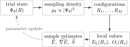
The VMC loop. For fixed $\theta$, configurations are sampled from $p_\theta\propto\lvert\Psi_\theta\rvert^2$ and converted into local estimates. Optimization then updates the trial state. Sampling error, optimization error, and ansatz bias enter at different stages.

Zero variance and the Schrödinger residual

The local-energy variance is

$$\sigma_{mathrm L}^2 = \left\langle \left\lvert E_{\mathrm L}-E\right\rvert^2 \right\rangle_{p_\theta}.$$

Substituting the definitions gives

$$\begin{aligned} \sigma_{\mathrm L}^2 &= \frac{1}{Z_\theta} \int dR\, \left\lvert (H-E)\Psi_\theta(R) \right\rvert^2 \\ &= \frac{ \left\lVert(H-E)\Psi_\theta\right\rVert^2 }{ \left\lVert\Psi_\theta\right\rVert^2 }. \end{aligned}$$

Thus the local-energy variance is the squared norm of the stationary Schrödinger residual, divided by the state norm. When $\Psi_\theta$ lies in the operator domain of $H$, this is also the usual energy variance.

If the trial state is an exact eigenstate,

$$H\Psi_\theta = E\Psi_\theta,$$

then

$$E_{\mathrm L}(R)=E$$

wherever the ratio is defined, and $\sigma_{\mathrm L}^2=0$. Conversely, a normalized pure state with zero residual variance is an eigenstate. This is the zero-variance principle.

The result is stronger than the statement that an eigenstate has the correct mean energy: every sampled configuration returns the same local energy. Near a good eigenstate, reduced local-energy fluctuations often make VMC statistically efficient.

Two cautions matter:

• A small energy error does not universally imply a proportionally small variance, or vice versa, without information about spectral gaps and state overlap.
• The Rayleigh quotient may be finite for a state in the quadratic-form domain even when $H\Psi$ is not square-integrable. In that case the energy exists but the local-energy variance can diverge.

Correct cusp, boundary, and nodal behavior is therefore both physical and statistical. It can remove singular cancellations that would otherwise create heavy local-energy tails.

Sampling the Born density

Independent samples from $p_\theta$ are rarely available in a complicated many-body problem. VMC commonly uses a Markov chain with stationary density $p_\theta$.

Given a proposal density $q(R'\mid R)$, the Metropolis–Hastings acceptance probability is

$$\begin{aligned} A(R\to R') = \min\left[ 1, \frac{ p_\theta(R')q(R\mid R') }{ p_\theta(R)q(R'\mid R) } \right]. \end{aligned}$$

For a symmetric proposal,

$$A(R\to R') = \min\left[ 1, \frac{\lvert\Psi_\theta(R')\rvert^2} {\lvert\Psi_\theta(R)\rvert^2} \right].$$

Normalization cancels from the ratio, so VMC does not require prior knowledge of $Z_\theta$. Detailed balance is a sufficient route to the desired stationary distribution, but stationarity alone is not enough: the chain must also explore every relevant region on the time scale of the calculation.

Nodes or separated modes can obstruct mixing. A local proposal may remain trapped in one nodal pocket or one metastable region even though its acceptance rate looks healthy. Acceptance rate is therefore not an ergodicity certificate.

Fermions and signs

For a fixed antisymmetric trial wavefunction, ordinary VMC samples the positive density $\lvert\Psi_\theta\rvert^2$. The fermionic sign or phase enters the local energy through amplitude ratios and derivatives, not through a fluctuating signed sampling weight. In this limited sense, evaluating a specified fermionic trial state does not have the same average-sign problem as many projection or path-integral methods.

The hard fermionic physics has not disappeared. The antisymmetry and nodal surface must be represented by the ansatz, and poor nodes can dominate the variational bias. Fixed-node projection is a separate approximation associated with diffusion Monte Carlo, not a property of VMC itself.

Energy estimator and uncertainty

After equilibration, suppose a chain provides configurations

$$R_1,R_2,\ldots,R_M.$$

The sample-mean energy estimator is

$$\widehat E_M = \frac{1}{M} \sum_{s=1}^M E_{\mathrm L}(R_s).$$

For a complex local energy, one normally reports the real part and separately checks that the sampled imaginary mean is statistically consistent with zero.

If the samples were independent and the variance finite, the standard error would scale as $\sigma_{\mathrm L}/\sqrt M$. Markov-chain samples are correlated, so the relevant quantity is the autocovariance of the real local-energy fluctuations. Let

$$\delta E_s = \operatorname{Re}E_{\mathrm L}(R_s)-E,$$

and define

$$C_k = \mathbb E[\delta E_s\delta E_{s+k}], \qquad \rho_k=\frac{C_k}{C_0}.$$

The integrated autocorrelation time is

$$\tau_{\mathrm{int}} = \frac{1}{2} + \sum_{k=1}^{\infty}\rho_k,$$

when the sum converges. For a long stationary chain,

$$\operatorname{Var}(\widehat E_M) \approx \frac{2\tau_{\mathrm{int}}\sigma_{\mathrm R}^2}{M} = \frac{\sigma_{\mathrm R}^2}{M_{\mathrm{eff}}},$$

with

$$\sigma_{\mathrm R}^2 = \operatorname{Var} \left(\operatorname{Re}E_{\mathrm L}\right), \qquad M_{\mathrm{eff}} = \frac{M}{2\tau_{\mathrm{int}}}.$$

For a real local energy, $\sigma_{\mathrm R}^2=\sigma_{\mathrm L}^2$. For a complex local energy, the residual norm also contains fluctuations of the imaginary part, whereas the quoted real-energy standard error does not.

The central-limit approximation requires adequate mixing and sufficiently light tails. If $E_{\mathrm L}$ has rare, extreme excursions or infinite variance, a familiar-looking standard error can be meaningless. Independent chains, trace diagnostics, blocking or batching, and tail inspection are not optional decorations.

The reusable probability theory and error-bar machinery are developed in Monte Carlo Basics. This page keeps the emphasis on what those quantities mean for a variational quantum state.

What remains of the upper bound?

For every fixed admissible trial state, the exact Rayleigh quotient obeys

$$E(\theta)\geq E_0.$$

The finite-sample estimate does not obey the inequality sample by sample. It has the form

$$\widehat E_M = E(\theta) + \delta_{\mathrm{stat}} + \delta_{\mathrm{eq}} + \delta_{\mathrm{impl}},$$

where statistical fluctuation, incomplete equilibration, and implementation error have no common one-sided sign. A reported VMC number can fall below $E_0$ even when the underlying variational energy is above it.

Calling a Monte Carlo estimate an “upper bound” is justified only after attaching a statistically and systematically defensible one-sided uncertainty statement. A symmetric one-standard-error interval is not a rigorous bound.

Optimization creates another subtlety. If many noisy estimates are compared and the smallest is selected, the winner is preferentially associated with a downward fluctuation. Reusing the same sample to optimize and to report the final energy can therefore produce selection bias. A fresh validation sample at the final parameters helps separate optimization noise from final estimation.

Worked example: Gaussian oscillator recast as VMC

The Variational Estimate for the Harmonic Oscillator owns the deterministic derivation. Here the same family is recast as a sampling problem.

Take

$$\psi_b(x) = \frac{1}{(\pi b^2)^{1/4}} \exp\left(-\frac{x^2}{2b^2}\right),$$

so that

$$p_b(x) = \frac{1}{\sqrt\pi b} \exp\left(-\frac{x^2}{b^2}\right).$$

For

$$H = -\frac{\hbar^2}{2m}\frac{d^2}{dx^2} + \frac{1}{2}m\omega^2x^2,$$

the local energy is

$$E_{\mathrm L}(x) = \frac{\hbar^2}{2mb^2} + \frac{1}{2} \left( m\omega^2- \frac{\hbar^2}{mb^4} \right)x^2.$$

Sampling $x$ from $p_b$ and using $\langle x^2\rangle=b^2/2$ gives

$$E(b) = \frac{\hbar^2}{4mb^2} + \frac{m\omega^2b^2}{4}.$$

Let

$$\ell=\sqrt{\frac{\hbar}{m\omega}}, \qquad s=\frac{b}{\ell}.$$

The exact ground-state width is $b=\ell$. At that point the coefficient of $x^2$ in $E_{\mathrm L}$ vanishes, so every sample returns

$$E_{\mathrm L}(x)=\frac{\hbar\omega}{2}.$$

For a nonoptimal width, the local energy fluctuates with $x^2$. Its exact variance is

$$\sigma_{\mathrm L}^2 = \frac{(\hbar\omega)^2}{8} \left(s^2-s^{-2}\right)^2.$$

This example displays all three layers cleanly. The family contains the exact ground state, the local-energy variance diagnoses the residual, and finite sampling estimates the same analytic Rayleigh quotient with a parameter-dependent error bar.

Energy gradients from samples

The deterministic geometry of parameter optimization is developed in Variational Parameters. VMC makes its gradients into covariance estimators.

For real parameters, define logarithmic derivatives

$$O_i(R) = \partial_i\ln\Psi_\theta(R).$$

Thus

$$\partial_i\Psi_\theta(R) = O_i(R)\Psi_\theta(R).$$

Assume $H$ is independent of $\theta$, the required derivatives can be moved through the integrals, and boundary terms are controlled. Differentiating the Rayleigh quotient and using self-adjointness gives

$$\partial_iE = 2\operatorname{Re} \left[ \left\langle O_i^*E_{\mathrm L}\right\rangle - \left\langle O_i^*\right\rangle \left\langle E_{\mathrm L}\right\rangle \right].$$

Equivalently,

$$\partial_iE = 2\operatorname{Re} \left\langle O_i^*(E_{\mathrm L}-E) \right\rangle.$$

For a real positive trial state, this reduces to twice the covariance of $O_i$ and $E_{\mathrm L}$. The formula is valuable because it does not require a separate pointwise derivative of $E_{\mathrm L}$: the Hamiltonian’s self-adjointness has converted the derivative into a covariance.

Replacing the expectations by sample means produces a stochastic gradient. Its noise is correlated across parameters because every component uses the same configurations. Near an eigenstate, the factor $E_{\mathrm L}-E$ becomes small, reflecting the zero-variance principle.

Finite-sample covariance estimators can still be biased at order $1/M$, and adaptive reuse of samples complicates the error analysis. Gradient convergence should be checked separately from energy convergence.

Stochastic reconfiguration and natural gradient

The logarithmic derivatives also give the pullback of the projective state metric:

$$S_{ij} = \operatorname{Re} \left[ \langle O_i^*O_j\rangle - \langle O_i^*\rangle \langle O_j\rangle \right].$$

For any real vector $v^i$,

$$v^iS_{ij}v^j\geq0.$$

Null directions correspond to parameter combinations that do not change the physical ray to first order, such as redundant coordinates or pure normalization and phase changes.

A natural-gradient or stochastic-reconfiguration step solves schematically

$$S_{ij}\,\delta\theta^j = -\eta\,\partial_iE,$$

where $\eta$ controls the step size. This chooses a small change in the quantum state rather than a small change measured only by coordinate distance.

The same metric appears in imaginary-time projection and the Time-Dependent Variational Principle. Stochastic reconfiguration is therefore not merely a preconditioner chosen by convenience; in its ideal form it is a sampled state-space projection.

In practice, $S$ is itself noisy and often ill-conditioned. Gauge fixing, rank truncation, diagonal shifts, trust regions, or pseudoinverses may be needed. Every such regularization changes the update and should be included in sensitivity tests.

Other optimization strategies include direct stochastic gradients, variance minimization, and the linear method. No optimizer repairs a trial family that omits the relevant symmetry, nodes, correlations, or asymptotic behavior.

Trial-state design for VMC

A VMC ansatz must be physically admissible, but it must also make the sampled quantities tractable. Useful requirements include:

• inexpensive evaluation of amplitude ratios or logarithmic amplitudes;
• exact enforcement of required exchange symmetry and quantum numbers;
• correct boundary, cusp, and asymptotic behavior where known;
• stable derivatives for $E_{\mathrm L}$ and $O_i$;
• support broad enough to cover every relevant configuration sector;
• a parameterization whose metric is not needlessly singular.

Common continuum fermion states combine a Slater determinant with a symmetric Jastrow factor,

$$\Psi_\theta(R) = D_\theta(R)e^{J_\theta(R)}.$$

The determinant enforces antisymmetry, while the Jastrow factor represents symmetric correlations and can encode cusp conditions. Backflow coordinates, pairing determinants, and Pfaffian forms enrich the nodal and pairing structure.

On lattices, correlator products, projected mean-field states, tensor-network amplitudes, and neural-network wavefunctions can all be sampled when their amplitudes and local connections are evaluable. Expressivity is not a guarantee of accuracy: a larger family may be harder to mix, optimize, condition, and validate.

Neural quantum states are therefore best viewed as flexible VMC ansätze, not as a separate variational theorem. Their claims require the same energy, variance, symmetry, convergence, and independent-benchmark checks as traditional trial states.

Observables beyond the energy

The local-estimator identity applies to any operator for which the expectation exists. For a Hermitian observable $A$,

$$\langle A\rangle_\theta = \left\langle A_{\mathrm L}\right\rangle_{p_\theta}.$$

Unlike the energy, a generic observable has no variational upper-bound property. It also need not be stationary to first order in the wavefunction error. A trial state can therefore have an excellent energy while giving a noticeably biased density, correlation function, response, or transition matrix element.

Variance and mixing are observable-dependent. A chain that estimates the energy efficiently may have a much longer autocorrelation time for a collective order parameter. Error bars must be computed for the observable actually reported.

Off-diagonal estimators may involve large amplitude ratios and heavier tails than the energy. Their finite variance should be checked rather than assumed.

Error budget

Let $\theta_\star$ minimize the exact variational energy within the chosen family, and let $\widehat\theta$ be the parameters returned by a noisy optimization. Then a useful conceptual decomposition is

$$\begin{aligned} \widehat E(\widehat\theta)-E_0 = {}& \underbrace{E(\theta_\star)-E_0}_{\text{ansatz bias}} \\ &+ \underbrace{E(\widehat\theta)-E(\theta_\star)} _{\text{optimization error}} \\ &+ \underbrace{\widehat E(\widehat\theta)-E(\widehat\theta)} _{\text{estimation error}}. \end{aligned}$$

For an exact global minimum within an admissible family, the first two terms are nonnegative. The last term has either sign and includes more than finite-sample variance if equilibration or implementation is imperfect.

A complete VMC error ledger separates:

• ansatz bias: the family cannot represent the target state;
• optimization error: the algorithm does not reach the best state in the family;
• sampling variance: a finite correlated sample fluctuates;
• equilibration and mixing bias: the chain does not represent $p_\theta$;
• estimator pathology: local values have heavy or nonintegrable tails;
• implementation error: derivatives, Hamiltonian terms, boundary conditions, or precision are wrong;
• model or discretization error: the simulated Hamiltonian differs from the intended physical problem.

Only sampling variance is expected to shrink automatically as $M^{-1/2}$ under ordinary central-limit conditions.

Minimum reporting standard

A trustworthy VMC result should report enough information to reconstruct the error logic:

• the Hamiltonian, boundary conditions, and sampled configuration space;
• the trial-state form, symmetry sector, parameter count, and optimization objective;
• the sampling distribution and proposal class;
• equilibration checks, chain lengths, independent-chain count, and autocorrelation or blocking analysis;
• the final energy with uncertainty and the local-energy variance;
• optimization convergence and regularization sensitivity;
• convergence under ansatz enlargement and comparison with independent benchmarks;
• separate validation samples when optimization and final estimation share data;
• random seeds and other reproducibility metadata in computational work.

An energy with many printed digits but no autocorrelation or ansatz-convergence evidence is not a high-precision result.

Boundary with computational methods

This preview establishes why the VMC estimators work and what their errors mean. A full computational treatment should own:

• stable determinant, Pfaffian, and neural-amplitude updates;
• proposal design and drift-diffusion sampling;
• burn-in, blocking, effective sample size, and convergence diagnostics;
• parallel and population sampling;
• robust stochastic-reconfiguration and linear-method solvers;
• automatic differentiation and custom local-energy kernels;
• correlated sampling and reweighting diagnostics;
• benchmark implementations with exact or independently converged answers.

Diffusion Monte Carlo, path-integral Monte Carlo, worldline methods, and auxiliary-field methods use different stochastic representations. They should not be inferred from the $\lvert\Psi_\theta\rvert^2$ sampling identity alone.

Common mistakes

• Treating $\widehat E_M$ as an exact upper bound. The underlying Rayleigh quotient is variational; its noisy estimate can fluctuate below $E_0$.
• Dividing the raw variance by $M$. Correlated samples require an autocorrelation correction or equivalent blocking analysis.
• Using acceptance rate as the only chain diagnostic. A chain can accept often while remaining trapped in one mode or nodal pocket.
• Ignoring local-energy tails. A finite-looking mean does not guarantee a finite or well-estimated variance.
• Dropping complex conjugation in the gradient. For complex trial states, the covariance uses $O_i^*$ and a final real part.
• Reusing optimization samples without acknowledging selection bias. Fresh final samples help separate fitting from evaluation.
• Calling every fermionic difficulty a sign problem. Fixed-state VMC samples a positive density, while nodal bias and projection-method sign problems are distinct issues.
• Optimizing only the energy mean. Variance, symmetries, observables, and ansatz convergence reveal failures hidden by a favorable energy.
• Regularizing the metric silently. A diagonal shift or rank cutoff changes the parameter update.
• Assuming a more expressive ansatz is automatically better. Expressivity can worsen conditioning, mixing, and optimization.

Exercises

1. Derive the local-estimator identity

Starting from the normalized expectation of an operator $A$, derive

$$\langle A\rangle_\theta = \int dR\,p_\theta(R)A_{\mathrm L}(R).$$

State the support caveat.

Solution

By definition,

$$\langle A\rangle_\theta = \frac{ \int dR\,\Psi_\theta^*(R)(A\Psi_\theta)(R) }{Z_\theta}.$$

Where $\Psi_\theta(R)\neq0$, multiply and divide the integrand by $\Psi_\theta(R)$:

$$\begin{aligned} \langle A\rangle_\theta &= \int dR\, \frac{\lvert\Psi_\theta(R)\rvert^2}{Z_\theta} \frac{(A\Psi_\theta)(R)}{\Psi_\theta(R)} \\ &= \int dR\,p_\theta(R)A_{\mathrm L}(R). \end{aligned}$$

The ratio is undefined at nodes. Nodes themselves have zero $p_\theta$ measure, but singular behavior near them must still be integrable for the mean and variance under discussion to exist.

2. Prove the zero-variance identity

Show that

$$\left\langle \left\lvert E_{\mathrm L}-E\right\rvert^2 \right\rangle_{p_\theta} = \frac{\lVert(H-E)\Psi_\theta\rVert^2} {\lVert\Psi_\theta\rVert^2}.$$

Why does zero variance imply an eigenstate?

Solution

Use

$$(E_{\mathrm L}-E)\Psi_\theta = (H-E)\Psi_\theta.$$

Then

$$\begin{aligned} \sigma_{\mathrm L}^2 &= \frac{1}{Z_\theta} \int dR\, \left\lvert (E_{\mathrm L}-E)\Psi_\theta \right\rvert^2 \\ &= \frac{1}{Z_\theta} \int dR\, \left\lvert(H-E)\Psi_\theta\right\rvert^2. \end{aligned}$$

Since $Z_\theta=\lVert\Psi_\theta\rVert^2$, the identity follows. A squared Hilbert-space norm vanishes only when its vector vanishes, so zero variance gives

$$(H-E)\Psi_\theta=0.$$

Thus a nonzero state in the operator domain is an eigenstate with eigenvalue $E$.

3. Oscillator mean and variance

For the Gaussian oscillator example, use

$$\langle x^2\rangle=\frac{b^2}{2}, \qquad \langle x^4\rangle=\frac{3b^4}{4}$$

to derive both $E(b)$ and $\sigma_{\mathrm L}^2$.

Solution

Write

$$E_{\mathrm L}(x)=A+Bx^2,$$

where

$$\begin{aligned} A&=\frac{\hbar^2}{2mb^2}, \\ B&=\frac{1}{2} \left( m\omega^2- \frac{\hbar^2}{mb^4} \right). \end{aligned}$$

The mean is

$$\begin{aligned} E(b) &=A+B\langle x^2\rangle \\ &= \frac{\hbar^2}{4mb^2} + \frac{m\omega^2b^2}{4}. \end{aligned}$$

The constant $A$ does not contribute to the variance, and

$$\operatorname{Var}(x^2) = \langle x^4\rangle-\langle x^2\rangle^2 = \frac{b^4}{2}.$$

Therefore

$$\begin{aligned} \sigma_{\mathrm L}^2 &=B^2\frac{b^4}{2} \\ &= \frac{1}{8} \left( m\omega^2b^2- \frac{\hbar^2}{mb^2} \right)^2 \\ &= \frac{(\hbar\omega)^2}{8} \left(s^2-s^{-2}\right)^2. \end{aligned}$$

4. Effective sample size for exponential correlation

Suppose $\rho_k=r^k$ with $0\leq r\lt1$. Compute $\tau_{\mathrm{int}}$ and $M_{\mathrm{eff}}$. What fraction of $M$ remains effective when $r=0.8$?

Solution

The geometric series gives

$$\begin{aligned} \tau_{\mathrm{int}} &= \frac{1}{2} + \sum_{k=1}^{\infty}r^k \\ &= \frac{1}{2} + \frac{r}{1-r} = \frac{1+r}{2(1-r)}. \end{aligned}$$

Hence

$$M_{\mathrm{eff}} = M\frac{1-r}{1+r}.$$

For $r=0.8$,

$$M_{\mathrm{eff}}=\frac{M}{9}.$$

Nine stored configurations then carry roughly the mean-estimation information of one independent draw, under this idealized correlation model.

5. Derive the covariance gradient

For real $\theta^i$, use $\partial_i\Psi=O_i\Psi$ to derive

$$\partial_iE = 2\operatorname{Re} \left[ \langle O_i^*E_{\mathrm L}\rangle - \langle O_i^*\rangle\langle E_{\mathrm L}\rangle \right].$$

Solution

Let

$$\begin{aligned} N&=\langle\Psi\rvert H\lvert\Psi\rangle, \\ Z&=\langle\Psi\vert\Psi\rangle, \qquad E=\frac{N}{Z}. \end{aligned}$$

Self-adjointness gives

$$\begin{aligned} \partial_iN &= \langle\partial_i\Psi\rvert H\lvert\Psi\rangle + \langle\Psi\rvert H\lvert\partial_i\Psi\rangle \\ &= 2Z\operatorname{Re} \langle O_i^*E_{\mathrm L}\rangle. \end{aligned}$$

Similarly,

$$\partial_iZ = 2Z\operatorname{Re}\langle O_i\rangle.$$

Differentiating $E=N/Z$ gives

$$\partial_iE = 2\operatorname{Re} \left[ \langle O_i^*E_{\mathrm L}\rangle -E\langle O_i^*\rangle \right].$$

Since the exact local-energy mean equals the real number $E$, this is the stated covariance form.

6. A sampled value below the ground-state energy

A VMC run returns $\widehat E=-1.01$ with estimated standard error $0.03$, while the exact ground-state energy is known to be $E_0=-1$. Does this violate the variational principle? What should be checked?

Solution

No. The variational principle constrains the exact Rayleigh quotient $E(\theta)$ of the trial state, not every finite-sample realization $\widehat E$. The observed difference is only one third of the quoted standard error.

One should check that the error estimate accounts for autocorrelation, that the chain is equilibrated and mixing, that the local-energy variance is finite, and that no implementation or discretization bias is present. If the parameters were selected using the same noisy sample, a fresh validation run is also appropriate. Only a controlled one-sided confidence statement could turn the stochastic result into a probabilistic upper bound.

References

• W. L. McMillan, “Ground State of Liquid He4,” Physical Review 138, A442–A451 (1965), doi:10.1103/PhysRev.138.A442.
• N. Metropolis, A. W. Rosenbluth, M. N. Rosenbluth, A. H. Teller, and E. Teller, “Equation of State Calculations by Fast Computing Machines,” Journal of Chemical Physics 21, 1087–1092 (1953), doi:10.1063/1.1699114.
• W. K. Hastings, “Monte Carlo sampling methods using Markov chains and their applications,” Biometrika 57, 97–109 (1970), doi:10.1093/biomet/57.1.97.
• D. M. Ceperley, G. V. Chester, and M. H. Kalos, “Monte Carlo simulation of a many-fermion system,” Physical Review B 16, 3081–3099 (1977), doi:10.1103/PhysRevB.16.3081.
• C. J. Umrigar, K. G. Wilson, and J. W. Wilkins, “Optimized trial wave functions for quantum Monte Carlo calculations,” Physical Review Letters 60, 1719–1722 (1988), doi:10.1103/PhysRevLett.60.1719.
• S. Sorella, “Wave function optimization in the variational Monte Carlo method,” Physical Review B 71, 241103(R) (2005), doi:10.1103/PhysRevB.71.241103.
• W. M. C. Foulkes, L. Mitas, R. J. Needs, and G. Rajagopal, “Quantum Monte Carlo simulations of solids,” Reviews of Modern Physics 73, 33–83 (2001), doi:10.1103/RevModPhys.73.33.
• G. Carleo and M. Troyer, “Solving the quantum many-body problem with artificial neural networks,” Science 355, 602–606 (2017), doi:10.1126/science.aag2302.