Upper Bounds and the Min–Max Principle

The ground-state variational principle is the first member of a hierarchy. The min–max principle characterizes every discrete eigenvalue below the essential spectrum by optimizing the Rayleigh quotient over subspaces of a prescribed dimension. It is the theorem behind excited-state Ritz bounds, eigenvalue interlacing, and the monotone improvement of finite-basis spectra.

The theorem is precise about what is bounded. Eigenvalues are ordered and counted with multiplicity; trial vectors must lie in the energy form domain; and the familiar upper-bound conclusion applies to discrete levels below the essential-spectrum threshold. A finite matrix always has discrete eigenvalues, but not every eigenvalue of a discretized continuum is an approximation to a bound state.

This page owns those guarantees and caveats. Matrix construction and diagonalization remain the canonical subject of the Rayleigh–Ritz Method, while the ground-state proof is given in the Variational Principle.

Setup and Spectral Ordering

Let $H$ be a self-adjoint Hamiltonian bounded from below. Denote its closed quadratic form by

$$q_H[\psi]$$

and its form domain by $\mathcal Q(H)$. For every nonzero $\psi\in\mathcal Q(H)$, define

$$\mathcal R_H[\psi] = \frac{q_H[\psi]}{ \lVert\psi\rVert^2 }.$$

When $\psi$ lies in the operator domain, this agrees with

$$\mathcal R_H[\psi] = \frac{ \langle\psi\rvert H\lvert\psi\rangle }{ \langle\psi\vert\psi\rangle }.$$

Let

$$\Sigma = \inf\sigma_{\mathrm{ess}}(H)$$

be the bottom of the essential spectrum, and write

$$E_{\mathrm{bot}} = \inf\sigma(H)$$

for the bottom of the full spectrum. List the discrete eigenvalues below $\Sigma$ as

$$E_0 \leq E_1 \leq E_2 \leq \cdots \lt \Sigma,$$

counting multiplicity. Thus a threefold-degenerate energy occupies three consecutive positions in the list.

If $H$ has compact resolvent, its spectrum is purely discrete with finite multiplicities and no finite accumulation point. One may then regard $\Sigma=+\infty$ for the purpose of this discussion. If essential spectrum is present, only finitely or countably many discrete levels may lie below its threshold.

Ground State as the First Min–Max Level

The bottom of the spectrum is characterized by

$$E_{\mathrm{bot}} = \inf_{ \substack{ \psi\in\mathcal Q(H)\\ \psi\ne0 } } \mathcal R_H[\psi].$$

If a discrete ground-state eigenvalue $E_0$ exists below $\Sigma$, then $E_{\mathrm{bot}}=E_0$ and a ground-state eigenvector attains the infimum. If the spectrum begins with continuum and has no bound state, then $E_{\mathrm{bot}}=\Sigma$ and the infimum need not be attained by any normalizable vector.

Restricting the search to a trial set $\mathcal T\subset\mathcal Q(H)$ gives

$$\inf_{ \substack{ \psi\in\mathcal T\\ \psi\ne0 } } \mathcal R_H[\psi] \geq E_{\mathrm{bot}}.$$

When a ground-state eigenvalue exists, this is the familiar upper bound to $E_0$. The higher-level theorem replaces a single trial vector by a trial subspace.

Exact Orthogonality and Excited States

Suppose exact orthonormal eigenvectors $\lvert0\rangle,\ldots,\lvert k-1\rangle$ for all lower indices are known. Define

$$\mathcal L_{k-1} = \operatorname{span} \{ \lvert0\rangle, \ldots, \lvert k-1\rangle \}.$$

Then

$$E_k = \inf_{ \substack{ \psi\in\mathcal Q(H)\\ \psi\ne0\\ \psi\perp\mathcal L_{k-1} } } \mathcal R_H[\psi].$$

To see why, expand an admissible normalized state orthogonal to the lower eigenspace:

$$\lvert\psi\rangle = \sum_{n\geq k} c_n\lvert n\rangle + \lvert\psi_{\mathrm{cont}}\rangle.$$

Every remaining spectral contribution has energy at least $E_k$, so

$$\mathcal R_H[\psi] \geq E_k.$$

The state $\lvert k\rangle$ attains equality. Degeneracy causes no problem when indices are counted with multiplicity and the lower subspace is specified consistently.

The formula is conceptually useful but computationally circular: if the exact lower eigenvectors were available, much of the spectral problem would already be solved.

Why Approximate Orthogonality Can Lose the Bound

Replacing exact lower states by approximate ones does not preserve the excited-state upper bound. A two-level system makes the failure explicit. Let

$$H = E_0\lvert0\rangle\langle0\rvert + E_1\lvert1\rangle\langle1\rvert, \qquad E_0\lt E_1.$$

Take an approximate ground state

$$\lvert\widetilde 0\rangle = \cos\varepsilon\lvert0\rangle + \sin\varepsilon\lvert1\rangle.$$

The unique normalized state orthogonal to it is, up to phase,

$$\lvert\chi\rangle = -\sin\varepsilon\lvert0\rangle + \cos\varepsilon\lvert1\rangle.$$

Its energy is

$$\begin{aligned} \mathcal R_H[\chi] ={}& E_0\sin^2\varepsilon + E_1\cos^2\varepsilon \\ ={}& E_1 - (E_1-E_0) \sin^2\varepsilon. \end{aligned}$$

For $\varepsilon\ne0$, this lies below $E_1$. Orthogonality to an inaccurate ground state leaves a component of the true ground state in the putative excitation.

Penalty methods need the same care. Minimizing

$$H_\Lambda = H + \Lambda \lvert\widetilde0\rangle \langle\widetilde0\rvert$$

is a variational problem for the modified Hamiltonian $H_\Lambda$. Its ground energy is not automatically an upper bound to $E_1$ of the original $H$.

Exact symmetry sectors are different. If $H$ preserves a subspace with quantum number $q$, minimization in that invariant sector bounds its lowest energy even when that state is excited relative to the full Hilbert space.

Courant–Fischer in Finite Dimension

Let $H$ be Hermitian on an $n$-dimensional Hilbert space, with ordered eigenvalues

$$E_0 \leq E_1 \leq \cdots \leq E_{n-1}.$$

For $k=0,\ldots,n-1$, the min–max formula is

$$E_k = \min_{ \substack{ \mathcal S\subset\mathcal H\\ \dim\mathcal S=k+1 } } \; \max_{ \substack{ \psi\in\mathcal S\\ \psi\ne0 } } \mathcal R_H[\psi].$$

An equivalent max–min formula is

$$E_k = \max_{ \substack{ \mathcal M\subset\mathcal H\\ \dim\mathcal M=k } } \; \min_{ \substack{ \psi\perp\mathcal M\\ \psi\ne0 } } \mathcal R_H[\psi].$$

The first form says: among all $(k+1)$-dimensional subspaces, choose the one whose highest Rayleigh quotient is as low as possible. The optimal choice is the exact low-energy subspace

$$\mathcal S_k = \operatorname{span} \{ \lvert0\rangle, \ldots, \lvert k\rangle \}.$$

Proof of the min–max form

For $\mathcal S_k$, every normalized vector has energy no greater than $E_k$, and $\lvert k\rangle$ has energy $E_k$. Therefore

$$\max_{ \psi\in\mathcal S_k\setminus\{0\} } \mathcal R_H[\psi] = E_k.$$

This proves that the min–max value is at most $E_k$.

Now take any subspace $\mathcal S$ of dimension $k+1$. The lower exact subspace

$$\mathcal L_{k-1} = \operatorname{span} \{ \lvert0\rangle, \ldots, \lvert k-1\rangle \}$$

has dimension $k$. Dimension counting implies that $\mathcal S$ contains a nonzero vector orthogonal to $\mathcal L_{k-1}$. That vector has Rayleigh quotient at least $E_k$. Hence

$$\max_{ \psi\in\mathcal S\setminus\{0\} } \mathcal R_H[\psi] \geq E_k.$$

Since this is true for every $(k+1)$-dimensional $\mathcal S$, the minimum of those maxima is at least $E_k$. The two inequalities prove the formula.

Semibounded-Operator Min–Max Principle

For the self-adjoint, semibounded operator introduced above, define the $k$th variational level

$$\mu_k(H) = \inf_{ \substack{ \mathcal S\subset\mathcal Q(H)\\ \dim\mathcal S=k+1 } } \; \sup_{ \substack{ \psi\in\mathcal S\\ \psi\ne0 } } \mathcal R_H[\psi].$$

For every index for which the $k$th discrete eigenvalue exists below the essential spectrum, the theorem states

$$\mu_k(H) = E_k.$$

The discrete eigenvalues are counted with multiplicity. If exactly $m$ such levels exist, then

$$\mu_k(H) = \Sigma, \qquad k\geq m.$$

If the resolvent is compact, the discrete case supplies the whole spectrum and $E_k\to+\infty$ as $k\to\infty$.

The second case is crucial. Variational levels do not enumerate a continuum as a sequence of normalizable eigenstates. Once no further discrete level exists below $\Sigma$, the min–max construction reaches the continuum threshold.

Ritz Values as Upper Bounds

Let $\mathcal V_N\subset\mathcal Q(H)$ be an $N$-dimensional trial subspace. Its ordered Ritz values

$$\vartheta_0^{(N)} \leq \vartheta_1^{(N)} \leq \cdots \leq \vartheta_{N-1}^{(N)}$$

have the internal variational characterization

$$\vartheta_k^{(N)} = \min_{ \substack{ \mathcal S\subset\mathcal V_N\\ \dim\mathcal S=k+1 } } \; \max_{ \substack{ \psi\in\mathcal S\\ \psi\ne0 } } \mathcal R_H[\psi].$$

The candidate subspaces are restricted to $\mathcal V_N$, so their minimum cannot be lower than the unrestricted one:

$$\vartheta_k^{(N)} \geq \mu_k(H).$$

Therefore, for every $0\leq k\leq N-1$ such that $E_k\lt\Sigma$ is a discrete eigenvalue,

$$\vartheta_k^{(N)} \geq E_k.$$

This is often called the Hylleraas–Undheim–MacDonald theorem in quantum chemistry. It avoids explicit orthogonality to unknown exact lower states: diagonalization optimizes all ordered states in the trial subspace simultaneously.

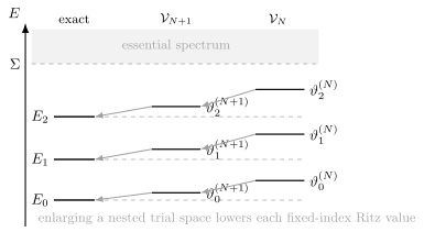
For nested trial spaces $\mathcal V_N\subset\mathcal V_{N+1}$, each fixed-index Ritz value can only decrease, while remaining above the corresponding discrete eigenvalue $E_k$ below the essential-spectrum threshold $\Sigma$.

Matrix realization

For a basis $\{\lvert\phi_i\rangle\}_{i=1}^N$, define

$$H_{ij} = \langle\phi_i\rvert H\lvert\phi_j\rangle, \qquad S_{ij} = \langle\phi_i\vert\phi_j\rangle.$$

The Ritz values are the generalized eigenvalues of

$$Hc = \vartheta Sc,$$

provided $S$ is positive definite on the retained span. Solving this finite problem accurately is the implementation; the min–max theorem explains its spectral ordering and bound.

Nested Spaces and Interlacing

If

$$\mathcal V_N \subset \mathcal V_{N+1},$$

then, for every fixed index available in both spaces,

$$\vartheta_k^{(N+1)} \leq \vartheta_k^{(N)}.$$

The larger space offers every old $(k+1)$-dimensional candidate subspace and additional ones, so the minimum cannot increase.

When the dimension increases by one, the sharper interlacing relation is

$$\vartheta_k^{(N+1)} \leq \vartheta_k^{(N)} \leq \vartheta_{k+1}^{(N+1)},$$

for $k=0,\ldots,N-1$. Thus new Ritz values enter between old ones while each fixed-index upper bound moves downward or stays fixed.

Monotonicity requires genuinely nested spaces and exact evaluation of the same Hamiltonian form. Changing a box, pseudopotential, quadrature rule, nonlinear basis family, or truncation prescription can destroy the set inclusion needed by the argument.

When Ritz Values Converge

Upper bounds need not be useful bounds. A sequence can remain far above the exact level. For nested spaces $\mathcal V_N$, convergence to a discrete eigenvalue follows under appropriate approximation hypotheses, commonly expressed by requiring the union of the spaces to be dense in the form domain with the form norm, or at least to approximate the relevant eigenspace in that norm.

Under such conditions, for every fixed discrete level below $\Sigma$,

$$\vartheta_k^{(N)} \downarrow E_k$$

as $N\to\infty$.

Density only in the Hilbert-space norm can be too weak for an unbounded Hamiltonian because it need not control kinetic energy or other contributions to the quadratic form.

Eigenvectors and degenerate clusters

Eigenvalue convergence does not imply that an individual Ritz vector has a stable identity. Near a degeneracy, numerical eigenvectors can rotate arbitrarily inside the nearly degenerate invariant subspace. Compare spectral projectors, subspace angles, symmetry labels, and matrix elements rather than component-by-component eigenvectors.

Residuals Add Local Spectral Information

Let $\lvert u\rangle\in\mathcal D(H)$ be a normalized Ritz vector with Ritz value $\vartheta$ and strong residual

$$\lvert r\rangle = (H-\vartheta) \lvert u\rangle.$$

For self-adjoint $H$, the spectral theorem implies

$$\operatorname{dist} \bigl( \vartheta, \sigma(H) \bigr) \leq \lVert r\rVert.$$

Thus a small residual guarantees that some spectral point lies nearby. It does not by itself identify the eigenvalue index, distinguish a discrete state from continuum, or certify that two nearly degenerate Ritz vectors span the correct subspace.

If $\mathcal V_N\subset\mathcal D(H)$, Ritz stationarity makes this residual orthogonal to the trial subspace:

$$\langle v\vert r\rangle = 0, \qquad v\in\mathcal V_N.$$

This Galerkin orthogonality says that the trial-space component of the eigen-equation error has been removed. The residual can still be large in directions absent from $\mathcal V_N$.

For a form-conforming space contained only in $\mathcal Q(H)$, the corresponding statement is instead

$$q_H[v,u] - \vartheta \langle v\vert u\rangle = 0, \qquad v\in\mathcal V_N.$$

A norm-valued strong residual need not exist until additional regularity places $u$ in $\mathcal D(H)$.

Numerical algorithms and residual stopping criteria are treated in Sparse Eigensolvers.

Degeneracy and Symmetry Sectors

Suppose

$$E_k = E_{k+1} = \cdots = E_{k+d-1}.$$

The energy has multiplicity $d$. A trial space must contain enough independent directions to approximate the whole eigenspace if all $d$ Ritz values are to converge. Capturing one linear combination does not certify the full degeneracy.

If a symmetry operator commutes with $H$, decompose the Hilbert space into invariant sectors and apply the min–max principle to each restricted Hamiltonian. The sector ground state is then the first min–max level in that sector. This is often the cleanest way to target an excited state with known parity, angular momentum, particle number, or another exact quantum number.

The ordering must be interpreted within the declared sector. The second state in one symmetry sector need not be the second state of the full spectrum.

Essential Spectrum and Continuum Caveats

The threshold $\Sigma$ is not decorative. It marks where the ordinary below-threshold min–max sequence stops identifying isolated bound states.

Finite boxes create pseudostates

Putting a scattering problem in a finite box replaces continuum by a discrete box spectrum. Those box eigenvalues are genuine eigenvalues of the finite-box Hamiltonian, but they are not upper bounds to a sequence of continuum eigenvalues of the infinite-volume operator. Their dependence on box size and boundary conditions must be analyzed separately.

Spectral pollution in gaps

For operators with gaps in the essential spectrum, naive Galerkin approximations can produce stable-looking Ritz values that converge to no true spectral point. This is spectral pollution. The below-threshold semibounded min–max theorem does not justify arbitrary interior-gap approximations.

Resonances are not ordinary eigenvalues

Metastable resonances generally are not normalizable eigenstates of the self-adjoint Hamiltonian. Complex scaling, analytic continuation, scattering poles, and stabilization methods have different variational structures; the ordinary real upper-bound theorem does not apply to a complex resonance energy.

Operators unbounded on both sides

The standard energy min–max principle assumes a lower-semibounded operator. The Dirac Hamiltonian is unbounded above and below, so naive energy minimization suffers variational collapse. Gap eigenvalues require specialized min–max constructions, spectral projections, or well-defined effective Hamiltonians.

Discretization can lose the bound

If matrix elements are approximated inconsistently, quadrature is biased, the overlap matrix is truncated, or the discretized form is not the restriction of the original form, a computed value need not remain an upper bound. A solver’s floating-point eigenvalue is a theorem about its matrix only after numerical error is controlled.

The operator, domain, and spectral distinctions used here are developed in Eigenvalue Problems, Unbounded Operators, and the Practical Spectral Theorem. Spatial discretization and spectral pollution are discussed in PDE Solvers.

A Three-Level Example

Let

$$\begin{aligned} H\lvert0\rangle &= 0, \\ H\lvert1\rangle &= \Delta\lvert1\rangle, \\ H\lvert2\rangle &= 3\Delta\lvert2\rangle, \end{aligned}$$

with $\Delta\gt0$. Choose the two-dimensional trial space

$$\mathcal V_2 = \operatorname{span} \left\{ \lvert1\rangle, \cos\alpha\lvert0\rangle + \sin\alpha\lvert2\rangle \right\}.$$

The two spanning vectors are orthonormal, and $H$ has no matrix element between them. The projected eigenvalues are therefore the ordered pair formed from

$$\Delta \qquad\text{and}\qquad 3\Delta\sin^2\alpha.$$

Hence

$$\vartheta_0^{(2)} = \min \left\{ \Delta, 3\Delta\sin^2\alpha \right\},$$ $$\vartheta_1^{(2)} = \max \left\{ \Delta, 3\Delta\sin^2\alpha \right\}.$$

The ordered bounds hold for every $\alpha$:

$$\vartheta_0^{(2)} \geq E_0=0, \qquad \vartheta_1^{(2)} \geq E_1=\Delta.$$

At values of $\alpha$ where the two projected energies cross, the labels attached to the basis vectors exchange, but the ordered Ritz indices remain the correct objects for the theorem.

What an Upper Bound Does Not Supply

The inequality

$$E_k \leq \vartheta_k^{(N)}$$

does not give a two-sided error bar. A lower bound, a gap estimate, a residual theorem, or an independently converged computation is needed to bracket the exact level.

As one example, Temple’s inequality can provide a ground-state lower bound from an energy expectation, its variance, and reliable information about the next spectral level. Its assumptions are additional information; it is not a consequence of the upper-bound statement alone.

Agreement of two Ritz calculations is strongest when the spaces are nested, matrix elements are independently checked, residuals are small, and the common limit lies safely below a known essential-spectrum threshold.

Practical Workflow

1. Specify the self-adjoint Hamiltonian, its boundary conditions, and the quadratic-form domain.
2. Identify the symmetry sector and whether the target lies below essential spectrum.
3. Order exact and approximate levels consistently, counting multiplicity.
4. Choose an admissible trial subspace and verify that its overlap matrix is positive definite on the retained span.
5. Solve the Hermitian generalized eigenproblem and sort the Ritz values.
6. Refine through nested spaces when possible and check fixed-index monotonicity.
7. Report residual norms and monitor invariant subspaces near degeneracies.
8. Vary box size, mesh, quadrature, and boundary conditions separately from basis enrichment.
9. Do not interpret above-threshold pseudostates or interior-gap values using the below-threshold theorem.

Common Mistakes

• Applying the ground-state upper bound to an excited-state ansatz without exact orthogonality, symmetry restriction, or min–max structure.
• Orthogonalizing against approximate lower states and assuming the resulting energy remains above the exact excitation.
• Forgetting that eigenvalues are counted with multiplicity.
• Comparing states by labels rather than sorting the Ritz spectrum consistently through crossings.
• Calling a sequence monotone when the trial spaces, Hamiltonian, box, or quadrature change together.
• Assuming Hilbert-norm density automatically controls an unbounded Hamiltonian’s quadratic form.
• Treating every finite-box level as a bound-state approximation.
• Reporting a stabilized Ritz value without its residual.
• Ignoring spectral pollution in gaps of essential spectrum.
• Applying ordinary energy minimization to an operator unbounded below.

Exercises

1. Prove finite-dimensional min–max

For a Hermitian matrix with ordered eigenvalues $E_0\leq\cdots\leq E_{n-1}$, prove

$$E_k = \min_{ \dim\mathcal S=k+1 } \max_{ \psi\in\mathcal S\setminus\{0\} } \mathcal R_H[\psi].$$

Solution

Choose

$$\mathcal S_k = \operatorname{span} \{ \lvert0\rangle, \ldots, \lvert k\rangle \}.$$

Every normalized vector in this subspace has Rayleigh quotient at most $E_k$, and $\lvert k\rangle$ attains $E_k$. Therefore the min–max value is at most $E_k$.

For any other $(k+1)$-dimensional subspace $\mathcal S$, dimension counting gives a nonzero vector in

$$\mathcal S \cap \operatorname{span} \{ \lvert0\rangle, \ldots, \lvert k-1\rangle \}^{\perp}.$$

That vector has support only on eigenvectors with index at least $k$, so its quotient is at least $E_k$. Hence the maximum over $\mathcal S$ is at least $E_k$. Taking the minimum over all $\mathcal S$ proves the equality.

2. Approximate orthogonality counterexample

For the two-level construction in the text, compute the energy of the state orthogonal to $\lvert\widetilde0\rangle$ and show explicitly how far it lies below $E_1$.

Solution

The orthogonal state is

$$\lvert\chi\rangle = -\sin\varepsilon\lvert0\rangle + \cos\varepsilon\lvert1\rangle.$$

Its energy is

$$\mathcal R_H[\chi] = E_0\sin^2\varepsilon + E_1\cos^2\varepsilon.$$

Therefore

$$E_1- \mathcal R_H[\chi] = (E_1-E_0) \sin^2\varepsilon.$$

Any nonzero error angle produces a value below the true excited energy. The violation is second order for small $\varepsilon$.

3. Analyze the three-level trial space

Derive the two Ritz values for $\mathcal V_2$ in the worked example. For which $\alpha$ do the two projected energies cross?

Solution

In the stated orthonormal basis, the projected Hamiltonian is diagonal:

$$H_{\mathcal V_2} = \begin{pmatrix} \Delta & 0 \\ 0 & 3\Delta\sin^2\alpha \end{pmatrix}.$$

The ordered eigenvalues are the minimum and maximum of the two diagonal entries. They cross when

$$3\Delta\sin^2\alpha = \Delta,$$

or

$$\sin^2\alpha = \frac13.$$

The basis-vector identity of the lower Ritz state changes there, while the ordered upper-bound statement remains valid.

4. Monotonicity under nested enrichment

Use the subspace min–max formula to prove that $\vartheta_k^{(N+1)}\leq\vartheta_k^{(N)}$ whenever $\mathcal V_N\subset\mathcal V_{N+1}$.

Solution

The value $\vartheta_k^{(N)}$ minimizes the largest Rayleigh quotient over all $(k+1)$-dimensional subspaces contained in $\mathcal V_N$. Every such subspace is also contained in $\mathcal V_{N+1}$. The larger trial space offers at least the same candidates and possibly better ones. Therefore

$$\vartheta_k^{(N+1)} \leq \vartheta_k^{(N)}.$$

No statement about convergence rate follows from this ordering alone.

5. Residual distance to the spectrum

Let $H$ be self-adjoint, $\lVert u\rVert=1$, $\vartheta=\langle u\rvert H\lvert u\rangle$, and $r=(H-\vartheta)u$. Use the spectral measure of $u$ to prove

$$\operatorname{dist} \bigl( \vartheta, \sigma(H) \bigr) \leq \lVert r\rVert.$$

Solution

Let $d\mu_u(E)$ be the normalized spectral measure of $u$. Then

$$\lVert r\rVert^2 = \int_{\sigma(H)} (E-\vartheta)^2 \,d\mu_u(E).$$

If every spectral point were farther than $\lVert r\rVert$ from $\vartheta$, then the integrand would be strictly greater than $\lVert r\rVert^2$ everywhere on the support of a probability measure. Its integral would then be strictly greater than $\lVert r\rVert^2$, a contradiction. Hence at least one spectral point lies within the residual norm.

6. Exhausting discrete levels

Suppose $H$ has exactly two discrete eigenvalues $E_0\leq E_1\lt\Sigma$ below its essential spectrum. What are $\mu_0(H)$, $\mu_1(H)$, and $\mu_2(H)$? Why does $\mu_2$ not identify a third bound state?

Solution

The min–max theorem gives

$$\mu_0(H) = E_0, \qquad \mu_1(H) = E_1.$$

After the two discrete levels are exhausted,

$$\mu_2(H) = \Sigma.$$

The value $\Sigma$ is the bottom of essential spectrum. It need not be a normalizable eigenvalue, so the third variational level marks the continuum threshold rather than a third bound state.

References

1. R. Courant and D. Hilbert, Methods of Mathematical Physics, Vol. I (Wiley-Interscience, 1989 reprint), chapters on eigenvalue problems and variational principles.
2. M. Reed and B. Simon, Methods of Modern Mathematical Physics, Vol. IV: Analysis of Operators (Academic Press, 1978), especially the min–max principle and Schrödinger-operator applications. Bibliographic record.
3. T. Kato, Perturbation Theory for Linear Operators, 2nd ed. (Springer, 1995), for closed forms, self-adjoint operators, and spectral approximation foundations.
4. J. K. L. MacDonald, “Successive Approximations by the Rayleigh–Ritz Variation Method”, Physical Review 43, 830–833 (1933). A classic derivation of successive Ritz bounds.
5. E. B. Davies, Spectral Theory and Differential Operators (Cambridge University Press, 1995), for discrete spectra, essential spectra, and variational eigenvalue methods.
6. I. Babuška and J. Osborn, “Eigenvalue Problems,” in Handbook of Numerical Analysis, Vol. II (North-Holland, 1991), pp. 641–787. A systematic treatment of variational spectral approximation.
7. M. Levitin and E. Shargorodsky, “Spectral pollution and second-order relative spectra for self-adjoint operators”, IMA Journal of Numerical Analysis 24, 393–416 (2004). A rigorous discussion of spurious Galerkin spectrum.