Gaussian Variational Methods

Gaussian trial states turn many infinite-dimensional variational calculations into finite-dimensional matrix problems. Their normalization, Fourier transforms, derivatives, overlaps, and polynomial moments are analytic. A positive-definite width matrix can represent anisotropy and coordinate correlations, while linear combinations of Gaussians can be enlarged systematically.

The convenience has a cost. A single Gaussian is nodeless, has a Gaussian tail, and has no Coulomb cusp. It can be exact for quadratic Hamiltonians and useful near smooth minima, but it can be structurally wrong for weak binding, tunneling between distant wells, singular interactions, or excited states. The variational theorem preserves an upper bound; it does not erase those ansatz limitations.

This page is the canonical home for static coordinate-space Gaussian variational ansätze. Gaussian probability integrals belong to Gaussian Distributions, Gaussian Wigner functions and symplectic spectra belong to Gaussian States Preview, and propagating complex-width packets belong to the Time-Dependent Variational Principle.

The complete one-dimensional quartic calculation, including optimization, upper-bound diagnostics, and numerical comparison, is Anharmonic Oscillator by Variational Methods.

When the Gaussian width is used as an adjustable reference frequency inside an order-by-order re-expansion, the method becomes Variational Perturbation Theory. Its first order reproduces a Gaussian Rayleigh quotient; higher orders are reorganized perturbative approximants and need not remain upper bounds.

Why Gaussians Are Useful

Several closure properties make Gaussians unusually tractable.

• Differentiating a Gaussian produces a polynomial times the same Gaussian.
• Multiplying two Gaussians produces another Gaussian times a constant.
• Fourier transformation maps a Gaussian to a Gaussian.
• Every polynomial moment follows from the covariance matrix by pairwise contractions.
• Multidimensional normalization reduces to a determinant.
• Positive-definite width matrices have stable factorizations and clear geometric meaning.

These properties make kinetic-energy matrix elements, harmonic potentials, polynomial interactions, and Gaussian-basis overlaps analytic. They are why Gaussian orbitals dominate much of molecular electronic-structure work and why correlated Gaussians are powerful in few-body calculations.

Analytic integrals are not the same as physical adequacy. The trial family must still represent the target state’s symmetry, scales, nodes, correlations, and asymptotic behavior.

General Real Gaussian Ansatz

Let

$$\mathbf x \in \mathbb R^d$$

collect $d$ Cartesian or internal coordinates, and let $A$ be a real symmetric positive-definite $d\times d$ matrix. With

$$\mathbf y = \mathbf x-\mathbf q,$$

define

$$\begin{aligned} \psi_{A,\mathbf q}(\mathbf x) ={}& \left( \frac{\det A}{\pi^d} \right)^{1/4} \\ &\times \exp\left[ -\frac12 \mathbf y^{\mathsf T}A\mathbf y \right]. \end{aligned}$$

The center is $\mathbf q$. The matrix $A$ is a precision matrix for the wavefunction amplitude; its eigenvalues have dimensions of inverse length squared. Positive definiteness ensures decay in every coordinate direction and makes the state normalizable.

Then the probability density is

$$\lvert\psi_{A,\mathbf q}(\mathbf x)\rvert^2 = \frac{\sqrt{\det A}}{\pi^{d/2}} e^{-\mathbf y^{\mathsf T}A\mathbf y}.$$

The multidimensional Gaussian integral

$$\int_{\mathbb R^d} e^{-\mathbf y^{\mathsf T}A\mathbf y} \,d^d y = \frac{\pi^{d/2}}{\sqrt{\det A}}$$

confirms normalization.

Width Matrix and Covariance

The position mean is

$$\langle\mathbf X\rangle = \mathbf q,$$

and the position covariance is

$$\Sigma_X = \left\langle (\mathbf X-\mathbf q) (\mathbf X-\mathbf q)^{\mathsf T} \right\rangle = \frac12A^{-1}.$$

Diagonalize the width matrix as

$$A = R \operatorname{diag}(a_1,\ldots,a_d) R^{\mathsf T},$$

where $R$ is orthogonal and every $a_j\gt0$. The columns of $R$ are the principal directions of the probability ellipsoid. Along principal direction $j$, the position standard deviation is

$$\sigma_j = \frac{1}{\sqrt{2a_j}}.$$

Off-diagonal entries of $A$ therefore have physical content: they rotate the principal axes and encode coordinate correlations. They are not merely inconvenient matrix elements to be discarded.

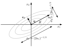
For $A=R\operatorname{diag}(a_1,a_2)R^{\mathsf T}$, the probability contours are ellipses whose principal standard deviations are $\sigma_j=(2a_j)^{-1/2}$. An off-diagonal entry in laboratory coordinates rotates the ellipse and permits correlations that a diagonal product ansatz cannot represent.

Width conventions

Three related matrices are easy to confuse:

Object	Matrix in the exponent	Position covariance
wavefunction amplitude	$A/2$	$A^{-1}/2$
probability density	$A$	$A^{-1}/2$
conventional normal density	$\Sigma_X^{-1}/2$	$\Sigma_X$

Since $\Sigma_X=A^{-1}/2$, the probability density can also be written

$$\begin{aligned} \lvert\psi\rvert^2 ={}& \frac{1}{ \sqrt{(2\pi)^d\det\Sigma_X} } \\ &\times \exp\left[ -\frac12 \mathbf y^{\mathsf T} \Sigma_X^{-1} \mathbf y \right]. \end{aligned}$$

Stating the convention is more reliable than calling every parameter simply a width.

Momentum Covariance and Kinetic Energy

For the real Gaussian,

$$\nabla\psi = -A\mathbf y\,\psi.$$

The momentum mean vanishes,

$$\langle\mathbf P\rangle = \mathbf 0,$$

and direct differentiation gives

$$\left\langle P_iP_j \right\rangle = \frac{\hbar^2}{2}A_{ij}.$$

Thus the momentum covariance matrix is

$$\Sigma_P = \frac{\hbar^2}{2}A.$$

In the principal basis,

$$\sigma_{x,j} = \frac{1}{\sqrt{2a_j}}, \qquad \sigma_{p,j} = \hbar\sqrt{\frac{a_j}{2}},$$

so every principal pair saturates

$$\sigma_{x,j}\sigma_{p,j} = \frac{\hbar}{2}.$$

Consider a kinetic energy with a symmetric positive-definite mass matrix $M$,

$$T = \frac12 \mathbf P^{\mathsf T} M^{-1} \mathbf P.$$

Its expectation is

$$\langle T\rangle_A = \frac{\hbar^2}{4} \operatorname{Tr} \left( M^{-1}A \right).$$

Large eigenvalues of $A$ describe narrow coordinate directions and increase the kinetic energy. This is the matrix version of the $b^{-2}$ localization cost in the harmonic-oscillator variational estimate.

Potential Expectations

For a coordinate-space potential,

$$\langle V\rangle_{A,\mathbf q} = \int_{\mathbb R^d} V(\mathbf x) \lvert\psi_{A,\mathbf q}(\mathbf x)\rvert^2 \,d^d x.$$

If $V$ is sufficiently regular and its Gaussian expectation exists, this is a Gaussian smoothing of the potential. For analytic $V$, it can be organized formally as

$$\langle V\rangle_{A,\mathbf q} = \left. \exp\left[ \frac14 \nabla^{\mathsf T} A^{-1} \nabla \right] V(\mathbf x) \right|_{\mathbf x=\mathbf q}.$$

The first terms are

$$\begin{aligned} \langle V\rangle_{A,\mathbf q} ={}& V(\mathbf q) \\ &+ \frac14 \operatorname{Tr} \left[ A^{-1} \nabla\nabla V(\mathbf q) \right] \\ &+ \text{higher even derivatives}. \end{aligned}$$

Odd centered moments vanish. Fourth moments obey the Gaussian pairing identity

$$\begin{aligned} \langle y_i y_j y_k y_\ell\rangle ={}& (\Sigma_X)_{ij}(\Sigma_X)_{k\ell} \\ &+ (\Sigma_X)_{ik}(\Sigma_X)_{j\ell} \\ &+ (\Sigma_X)_{i\ell}(\Sigma_X)_{jk}. \end{aligned}$$

This is the finite-dimensional Gaussian form of Wick or Isserlis pairing. It makes polynomial anharmonicities straightforward to evaluate, although their width optimization can still be nonlinear.

The center obeys a useful stationarity condition. Translating the normalized Gaussian gives

$$\frac{\partial E}{\partial q_i} = \left\langle \frac{\partial V}{\partial X_i} \right\rangle.$$

At an optimized center,

$$\langle\nabla V\rangle = \mathbf0.$$

This is an averaged force-balance equation, not generally the same as placing $\mathbf q$ at a pointwise minimum of $V$.

Exact Solution for Coupled Quadratic Hamiltonians

The matrix Gaussian becomes exact for a stable quadratic Hamiltonian. Let

$$\begin{aligned} H ={}& \frac12 \mathbf P^{\mathsf T}M^{-1}\mathbf P + V_0 \\ &+ \frac12 (\mathbf X-\mathbf q_0)^{\mathsf T} K (\mathbf X-\mathbf q_0), \end{aligned}$$

where both $M$ and $K$ are real symmetric positive-definite matrices.

The center is minimized at $\mathbf q=\mathbf q_0$. The Gaussian energy is

$$\begin{aligned} E(A) ={}& V_0 + \frac{\hbar^2}{4} \operatorname{Tr}(M^{-1}A) \\ &+ \frac14 \operatorname{Tr}(KA^{-1}). \end{aligned}$$

For a symmetric variation $\delta A$,

$$\delta A^{-1} = -A^{-1}(\delta A)A^{-1}.$$

Therefore

$$\begin{aligned} \delta E ={}& \frac14 \operatorname{Tr} \left[ \hbar^2M^{-1}\delta A \right] \\ &- \frac14 \operatorname{Tr} \left[ A^{-1}KA^{-1}\delta A \right]. \end{aligned}$$

Stationarity for every symmetric $\delta A$ requires

$$\hbar^2M^{-1} = A^{-1}KA^{-1},$$

or equivalently

$$\hbar^2 A M^{-1}A = K.$$

Define the mass-weighted force matrix

$$C = M^{-1/2}KM^{-1/2}.$$

Its positive square root gives the unique positive-definite stationary width,

$$A_\star = \frac{1}{\hbar} M^{1/2} C^{1/2} M^{1/2}.$$

The eigenvalues of $C^{1/2}$ are the normal-mode frequencies $\omega_j$. At the optimum,

$$\langle T\rangle_\star = \langle V-V_0\rangle_\star = \frac{\hbar}{4} \operatorname{Tr}(C^{1/2}),$$

and

$$E_\star = V_0 + \frac{\hbar}{2} \operatorname{Tr}(C^{1/2}) = V_0 + \frac{\hbar}{2} \sum_{j=1}^{d} \omega_j.$$

This is the exact coupled-oscillator ground energy. The full width matrix automatically performs the normal-mode rotation and assigns the correct width to every mode.

If $K$ has a zero or negative direction, the assumptions fail. A zero mode has no normalizable oscillator ground state in that coordinate, while a negative direction signals an unstable quadratic potential. The positive-definite solution should not be continued blindly through either case.

Worked Example: Two Coupled Coordinates

Consider equal masses with

$$\begin{aligned} H ={}& \frac{P_x^2+P_y^2}{2m} \\ &+ \frac{m}{2} \left[ \omega^2(x^2+y^2) + 2gxy \right], \end{aligned}$$

where

$$\lvert g\rvert \lt \omega^2$$

ensures stability. The normal coordinates are

$$q_+ = \frac{x+y}{\sqrt2}, \qquad q_- = \frac{x-y}{\sqrt2},$$

with frequencies

$$\omega_+ = \sqrt{\omega^2+g}, \qquad \omega_- = \sqrt{\omega^2-g}.$$

The exact Gaussian width matrix in the $(x,y)$ coordinates is

$$A_\star = \frac{m}{2\hbar} \begin{pmatrix} \omega_++\omega_- & \omega_+-\omega_- \\ \omega_+-\omega_- & \omega_++\omega_- \end{pmatrix}.$$

For $g\ne0$, the off-diagonal entry is nonzero. The exact ground state is correlated in the original coordinates even though it factorizes in the normal coordinates.

The exact energy is

$$E_0 = \frac{\hbar}{2} (\omega_++\omega_-).$$

Now restrict the trial family to an axis-aligned isotropic product,

$$\psi_a(x,y) = \left( \frac{a}{\pi} \right)^{1/2} e^{-a(x^2+y^2)/2}.$$

Because $\langle xy\rangle_a=0$, its energy is

$$E_{\mathrm{prod}}(a) = \frac{\hbar^2a}{2m} + \frac{m\omega^2}{2a}.$$

Optimization gives

$$a_\star = \frac{m\omega}{\hbar}, \qquad E_{\mathrm{prod},\star} = \hbar\omega.$$

For nonzero coupling,

$$\frac{\hbar}{2} \left( \sqrt{\omega^2+g} + \sqrt{\omega^2-g} \right) \lt \hbar\omega.$$

The restricted product misses correlation energy. Adding one off-diagonal width parameter is enough to recover the exact quadratic result.

Positive-Definite Parameterizations

Directly optimizing independent entries of $A$ can step outside the positive-definite cone, making the trial state nonnormalizable. A parameterization should enforce admissibility by construction.

Cholesky factor

Write

$$A = LL^{\mathsf T},$$

where $L$ is lower triangular and its diagonal entries are positive. Parameterize those diagonals as

$$L_{ii} = e^{\eta_i}.$$

This is efficient and guarantees $A\gt0$. The coordinates depend on the ordering and scaling of the original variables, so preprocessing still matters.

Matrix exponential

For any real symmetric matrix $S$,

$$A = e^S$$

is positive definite. This provides global unconstrained coordinates, although differentiating the matrix exponential is more expensive than differentiating a Cholesky factor.

Eigenvalues and rotations

The decomposition

$$A = R \operatorname{diag}(e^{\eta_1},\ldots,e^{\eta_d}) R^{\mathsf T}$$

is physically interpretable: the $\eta_j$ set principal widths and $R$ sets orientation. It becomes coordinate-singular when eigenvalues coincide because rotations inside a degenerate eigenspace do not change $A$.

Parameterization	Main advantage	Main caution
$A=LL^{\mathsf T}$	efficient and stable	coordinate-order dependence
$A=e^S$	unconstrained symmetric parameters	costly matrix derivatives
eigenvalues plus rotations	direct geometric meaning	redundant rotations at degeneracy

The normalization depends on $A$. The identity

$$\delta\log\det A = \operatorname{Tr} (A^{-1}\delta A)$$

is essential when differentiating normalized Gaussian states. Freezing the determinant prefactor produces the wrong energy gradient.

Complex Widths and Phase-Space Correlations

A more general pure Gaussian wave packet uses a real positive-definite amplitude matrix $A$, a real symmetric chirp matrix $B$, a center $\mathbf q$, and a mean momentum $\mathbf p$:

$$\begin{aligned} \psi_{A,B,\mathbf q,\mathbf p}(\mathbf x) ={}& \left( \frac{\det A}{\pi^d} \right)^{1/4} \\ &\times \exp\left[ -\frac12 \mathbf y^{\mathsf T}(A+iB)\mathbf y \right] \\ &\times \exp\left[ \frac{i}{\hbar} \mathbf p^{\mathsf T}\mathbf y \right]. \end{aligned}$$

The position covariance remains

$$\Sigma_X = \frac12A^{-1},$$

while the momentum covariance becomes

$$\Sigma_P = \frac{\hbar^2}{2} \left( A + B A^{-1}B \right).$$

The symmetrized position–momentum covariance block is

$$\Sigma_{XP} = -\frac{\hbar}{2} A^{-1}B.$$

Thus $B$ tilts the Gaussian in phase space and represents a quadratic phase or chirp. It is required for generic exact Gaussian dynamics even though it does not alter the position density at one instant.

For the static scalar Hamiltonian used above,

$$\begin{aligned} \langle T\rangle ={}& \frac12 \mathbf p^{\mathsf T}M^{-1}\mathbf p \\ &+ \frac{\hbar^2}{4} \operatorname{Tr} \left[ M^{-1} \left( A+B A^{-1}B \right) \right]. \end{aligned}$$

The $\mathbf p$ and $B$ contributions are nonnegative and do not change a coordinate-only potential expectation. In a time-reversal-invariant ground-state problem with no vector potential, their static optimum is therefore

$$\mathbf p_\star = \mathbf0, \qquad B_\star = 0.$$

Magnetic fields, imposed currents, angular momentum, and real-time propagation change that conclusion. The equations of motion for complex widths belong to the Time-Dependent Variational Principle, while covariance-matrix state classification belongs to Gaussian States Preview.

Squeezed-State Connection

A centered real Gaussian with a width different from a reference oscillator vacuum is a squeezed pure Gaussian state. In one dimension, if the reference precision is $a_0$ and

$$a = a_0e^{2r},$$

then

$$\frac{(\Delta X)^2}{(\Delta X)_0^2} = e^{-2r}, \qquad \frac{(\Delta P)^2}{(\Delta P)_0^2} = e^{2r}.$$

One quadrature narrows while its conjugate broadens. A multidimensional $A$ combines rotations and mode-dependent squeezing. This connection explains why Gaussian variational widths have a direct quantum-state interpretation, but it does not mean that every Gaussian variational problem should be reformulated in quantum-optics language. The canonical operator and noise discussion is in Squeezed States: First Encounter.

Linear Combinations of Gaussians

A single Gaussian is one nonlinear trial manifold. A Gaussian basis enlarges the state to

$$\Psi(\mathbf x) = \sum_{n=1}^{N} c_n \phi_n(\mathbf x),$$

where each $\phi_n$ may have its own center, width matrix, polynomial prefactor, and symmetry projection.

For fixed nonlinear Gaussian parameters, optimizing the coefficients gives the generalized eigenproblem

$$Hc = ESc.$$

An outer optimization then changes centers and width matrices. Separating the exact inner coefficient solve from the nonlinear outer search is usually more stable than treating all variables identically.

For two centered normalized real Gaussians, the overlap is

$$S(A,B) = \frac{ 2^{d/2} (\det A\det B)^{1/4} }{ \sqrt{\det(A+B)} }.$$

As $A$ and $B$ become nearly equal, their overlap approaches one. Large Gaussian bases can therefore develop near-linear dependence and an ill-conditioned overlap matrix.

Gaussian product theorem

For unnormalized one-dimensional functions,

$$g_{\alpha,A}(x) = e^{-\alpha(x-A)^2}.$$

Similarly,

$$g_{\beta,B}(x) = e^{-\beta(x-B)^2}.$$

Their product is

$$g_{\alpha,A}(x)g_{\beta,B}(x) = C_{AB} e^{-(\alpha+\beta)(x-P)^2},$$

where

$$P = \frac{\alpha A+\beta B}{\alpha+\beta}.$$

The separation-dependent factor is

$$C_{AB} = \exp\left[ -\frac{\alpha\beta}{\alpha+\beta} (A-B)^2 \right].$$

Products centered on different points reduce to one Gaussian centered at a weighted average. This identity is a major reason multicenter molecular integrals remain tractable.

Symmetry and Coordinate Choices

The basic centered Gaussian is even and nodeless. It is naturally suited to bosonic or spatial ground states, but not by itself to odd parity, nonzero angular momentum, or fermionic antisymmetry.

Common extensions include:

• multiplying by polynomials to create nodes and angular structure;
• projecting onto parity or rotational quantum numbers;
• antisymmetrizing products or using Slater determinants;
• combining displaced Gaussians to describe multiple centers;
• using explicitly correlated coordinates such as interparticle separations;
• separating center-of-mass and internal coordinates before optimizing widths.

For a translation-invariant many-particle Hamiltonian, a positive-definite Gaussian in all laboratory coordinates artificially localizes the free center of mass. Use Jacobi or other internal coordinates, or factor the center-of-mass motion explicitly. A singular width matrix in the full coordinate space does not define an ordinary normalized wavefunction there.

Coordinate scaling matters as well. If one coordinate is measured in ångströms and another represents a collective mode with a very different natural length, optimizing raw entries of $A$ can create severe conditioning problems. Mass weighting and nondimensionalization should precede nonlinear optimization.

Applications

Smooth confinement and local modes

Near a stable potential minimum, a quadratic Taylor expansion makes a Gaussian the natural first approximation. Anisotropic width matrices capture different normal-mode frequencies, and nonzero off-diagonal entries capture couplings in non-normal coordinates.

Molecular electronic structure

Gaussian-type orbitals make multicenter overlap, kinetic, and Coulomb integrals computationally tractable. Contracted Gaussian bases combine several primitive exponents to approximate physically better radial shapes. Fermionic antisymmetry and electron correlation still require determinants, configuration expansions, coupled-cluster methods, or explicitly correlated factors.

Few-body bound states

Correlated Gaussians in Jacobi coordinates can encode interparticle correlations through a full width matrix. Stochastic or deterministic selection of nonlinear widths, combined with exact coefficient optimization, gives systematically improvable calculations for atomic, molecular, nuclear, and other few-body systems.

Wave-packet and semiclassical dynamics

Centers, momenta, widths, and chirps form a finite-dimensional manifold for approximate dynamics. Quadratic Hamiltonians preserve the Gaussian family exactly; anharmonic evolution generates skewness, splitting, and higher cumulants that one Gaussian cannot retain. Static widths on this page become time-dependent coordinates in Gaussian wave-packet methods.

Mean-field models

Gaussian density profiles provide useful low-dimensional ansätze for trapped gases, nonlinear Schrödinger equations, and collective modes. Nonlinear interactions alter the width equation and can create collapse or multiple stationary branches, so positivity of $A$ alone does not guarantee a stable physical solution.

Limitations and Failure Modes

Wrong asymptotic tail

A Gaussian decays as

$$e^{-\alpha r^2},$$

faster than a typical short-range bound-state tail

$$e^{-\kappa r}.$$

This mismatch can strongly affect weak binding, tunneling amplitudes, polarizabilities, and large-distance observables even when the energy looks good.

Missing Coulomb cusp

At an electron–nucleus or electron–electron coalescence, the exact wavefunction satisfies a cusp relation. A smooth Gaussian centered at the coalescence has zero radial derivative there and cannot satisfy a nonzero cusp. Linear combinations can approximate the cusp, but convergence may be slow unless explicit correlation or cusp-corrected factors are included.

Nodes and sign structure

A single real Gaussian is positive everywhere. Excited states, fermionic states, and angular-momentum sectors require polynomial factors, symmetry projections, or signed combinations. Optimizing a nodeless Gaussian cannot discover a nodal surface absent from the ansatz.

Multimodal states

A state localized in two distant wells is poorly represented by one ellipse. A sum of displaced Gaussians can represent both lobes and their relative phase; a single covariance matrix cannot.

Nonlinear optimization and redundancy

Centers and widths create a nonconvex optimization problem. Permuting identical Gaussians leaves the state unchanged, coincident functions create nearly flat directions, and extreme widths can make matrix elements ill-conditioned. Report overlap spectra, gradient norms, multiple-start checks, and refinement stability.

Upper bounds do not validate observables

For an admissible normalized state and exact matrix elements, the energy remains an upper bound to the ground energy. A good bound does not certify tails, contact densities, transition amplitudes, or entanglement. Check observables that probe the physics the Gaussian family may miss.

Practical Workflow

1. Remove free center-of-mass motion and choose physically meaningful internal coordinates.
2. Identify exact symmetries, nodes, and required antisymmetry before choosing the Gaussian form.
3. Nondimensionalize coordinates and define the width convention explicitly.
4. Parameterize $A\gt0$ by Cholesky factors, a matrix exponential, or positive eigenvalues.
5. Evaluate normalization, moments, and matrix elements analytically where possible.
6. Optimize linear coefficients exactly for fixed nonlinear parameters.
7. Refine centers and widths while monitoring the overlap-matrix spectrum.
8. Check virial relations, residuals, local-energy variation, and independent observables.
9. Compare with a non-Gaussian family or a systematically enlarged Gaussian expansion.
10. Test asymptotic tails, cusp behavior, and symmetry explicitly rather than inferring them from the energy.

Common Mistakes

• Confusing the amplitude precision $A$ with the probability covariance $\Sigma_X=A^{-1}/2$.
• Optimizing unconstrained matrix entries and allowing $A$ to lose positive definiteness.
• Omitting the determinant-dependent normalization when differentiating widths.
• Forcing $A$ to be diagonal in coordinates where the Hamiltonian couples modes.
• Interpreting a rotated probability ellipse as a mixed state rather than a correlated pure wavefunction.
• Adding a complex chirp to a static scalar ground-state ansatz without checking its positive kinetic cost.
• Using a laboratory-coordinate Gaussian for a translation-invariant system without separating the center of mass.
• Treating a Gaussian basis as orthogonal and ignoring the condition number of its overlap matrix.
• Assuming many smooth Gaussians reproduce a cusp or exponential tail efficiently.
• Calling a converged Gaussian energy proof that all target observables have converged.

Exercises

1. Normalize the matrix Gaussian

For $A\gt0$, verify the normalization of $\psi_{A,\mathbf q}$ and derive

$$\Sigma_X = \frac12A^{-1}.$$

Solution

The squared normalization factor is

$$\left( \frac{\det A}{\pi^d} \right)^{1/2}.$$

After shifting to $\mathbf y=\mathbf x-\mathbf q$,

$$\int e^{-\mathbf y^{\mathsf T}A\mathbf y} \,d^dy = \frac{\pi^{d/2}}{\sqrt{\det A}}.$$

The two factors multiply to one.

Introduce a source $\mathbf J$:

$$Z(\mathbf J) = \int \exp\left( -\mathbf y^{\mathsf T}A\mathbf y + \mathbf J^{\mathsf T}\mathbf y \right) \,d^dy.$$

Completing the square gives

$$Z(\mathbf J) = Z(\mathbf0) \exp\left( \frac14 \mathbf J^{\mathsf T}A^{-1}\mathbf J \right).$$

Two source derivatives at $\mathbf J=0$ yield

$$\langle y_i y_j\rangle = \frac12(A^{-1})_{ij}.$$

Therefore $\Sigma_X=A^{-1}/2$.

2. Derive the kinetic trace

For

$$T = \frac12 \mathbf P^{\mathsf T}M^{-1}\mathbf P,$$

show that a centered real Gaussian satisfies

$$\langle T\rangle = \frac{\hbar^2}{4} \operatorname{Tr}(M^{-1}A).$$

Solution

Differentiation gives

$$\partial_i\psi = -(A\mathbf y)_i\psi,$$

and

$$\partial_i\partial_j\psi = \left[ (A\mathbf y)_i(A\mathbf y)_j - A_{ij} \right] \psi.$$

Using $\langle\mathbf y\mathbf y^{\mathsf T}\rangle=A^{-1}/2$,

$$\left\langle (A\mathbf y)_i(A\mathbf y)_j \right\rangle = \frac12A_{ij}.$$

Since $P_iP_j=-\hbar^2\partial_i\partial_j$,

$$\langle P_iP_j\rangle = \frac{\hbar^2}{2}A_{ij}.$$

Contracting with $(M^{-1})_{ij}/2$ gives the trace formula.

3. Solve the quadratic width equation

Starting from

$$\begin{aligned} E(A) ={}& V_0 + \frac{\hbar^2}{4} \operatorname{Tr}(M^{-1}A) \\ &+ \frac14 \operatorname{Tr}(KA^{-1}), \end{aligned}$$

derive the stationary equation and verify the stated positive-definite solution for $A_\star$.

Solution

Use

$$\delta A^{-1} = -A^{-1}(\delta A)A^{-1}.$$

Then

$$\delta E = \frac14 \operatorname{Tr} \left[ \left( \hbar^2M^{-1} - A^{-1}KA^{-1} \right) \delta A \right].$$

Stationarity for every symmetric variation gives

$$\hbar^2M^{-1} = A^{-1}KA^{-1},$$

or

$$\hbar^2AM^{-1}A = K.$$

Let

$$C = M^{-1/2}KM^{-1/2}$$

and propose

$$A_\star = \frac{1}{\hbar} M^{1/2}C^{1/2}M^{1/2}.$$

Substitution gives

$$\begin{aligned} \hbar^2A_\star M^{-1}A_\star &= M^{1/2}C M^{1/2} \\ &= K. \end{aligned}$$

All factors are positive definite, so this is the required admissible solution.

4. Quantify the missed correlation energy

For the two-coordinate example, expand the exact ground energy for small

$$\delta = \frac{g}{\omega^2}.$$

Compare it with the optimized isotropic product energy through order $\delta^2$.

Solution

The exact energy is

$$E_0 = \frac{\hbar\omega}{2} \left( \sqrt{1+\delta} + \sqrt{1-\delta} \right).$$

Using

$$\sqrt{1\pm\delta} = 1 \pm \frac{\delta}{2} - \frac{\delta^2}{8} \pm \frac{\delta^3}{16} + O(\delta^4),$$

the odd terms cancel:

$$E_0 = \hbar\omega \left[ 1 - \frac{\delta^2}{8} + O(\delta^4) \right].$$

The optimized isotropic product gives $E_{\mathrm{prod}}=\hbar\omega$. Its leading excess is therefore

$$E_{\mathrm{prod}}-E_0 = \frac{\hbar\omega}{8} \delta^2 + O(\delta^4).$$

The first missed contribution is quadratic because the cross expectation $\langle xy\rangle$ vanishes in the uncorrelated state.

5. Show that a static chirp costs kinetic energy

For the complex-width Gaussian, prove that the $B$-dependent kinetic contribution is nonnegative and determine when it vanishes.

Solution

The extra term is

$$\Delta T_B = \frac{\hbar^2}{4} \operatorname{Tr} \left( M^{-1}B A^{-1}B \right).$$

Define

$$D = A^{-1/2}BM^{-1/2}.$$

Then cyclicity of the trace gives

$$\Delta T_B = \frac{\hbar^2}{4} \operatorname{Tr} \left( DD^{\mathsf T} \right).$$

This is a Frobenius norm squared:

$$\Delta T_B = \frac{\hbar^2}{4} \left\lVert A^{-1/2}BM^{-1/2} \right\rVert_F^2 \geq 0.$$

Since $A$ and $M$ are invertible, it vanishes exactly when $B=0$.

6. Prove the Gaussian product theorem

Complete the square in

$$\alpha(x-A)^2 + \beta(x-B)^2$$

and derive the product center $P$ and the separation-dependent prefactor.

Solution

Let

$$S(x) = \alpha(x-A)^2 + \beta(x-B)^2.$$

Expanding gives

$$\begin{aligned} S(x) ={}& (\alpha+\beta)x^2 \\ &- 2(\alpha A+\beta B)x \\ &+ \alpha A^2+\beta B^2. \end{aligned}$$

Set

$$P = \frac{\alpha A+\beta B}{\alpha+\beta}.$$

Completing the square gives

$$\begin{aligned} S(x) ={}& (\alpha+\beta)(x-P)^2 \\ &+ \frac{\alpha\beta}{\alpha+\beta} (A-B)^2. \end{aligned}$$

Exponentiating the negative of both sides yields the theorem in the text.

References

1. R. Shankar, Principles of Quantum Mechanics, 2nd ed. (Springer, 1994), for the variational principle, oscillator, and Gaussian wave packets.
2. S. F. Boys, “Electronic wave functions. I. A general method of calculation for the stationary states of any molecular system”, Proceedings of the Royal Society A 200, 542–554 (1950), a foundational Gaussian-orbital construction.
3. Y. Suzuki and K. Varga, Stochastic Variational Approach to Quantum-Mechanical Few-Body Problems (Springer, 1998), for correlated Gaussian bases and nonlinear parameter selection.
4. T. Helgaker, P. Jørgensen, and J. Olsen, Molecular Electronic-Structure Theory (Wiley, 2000), for Gaussian basis functions, integral technology, and conditioning in electronic-structure calculations.
5. E. J. Heller, “Time-dependent approach to semiclassical dynamics”, Journal of Chemical Physics 62, 1544–1555 (1975), for evolving multidimensional Gaussian packets and complex width parameters.
6. C. Lubich, From Quantum to Classical Molecular Dynamics: Reduced Models and Numerical Analysis (European Mathematical Society, 2008), for variational Gaussian wave-packet dynamics and geometric numerical structure.