Common Variational Pitfalls

The variational principle is exact; a variational calculation can still be wrong. The usual failure is not a defect in the theorem but a mismatch between the theorem’s hypotheses and the quantity that was actually computed. A trial state may be inadmissible, a family may omit essential physics, an optimizer may stop at the wrong point, or a numerical estimator may not equal the Rayleigh quotient it is intended to approximate.

This page is the chapter’s diagnostic guide. It does not reprove the Variational Principle, repeat the construction of Trial Wavefunctions, or redevelop parameter gradients from Variational Parameters. Instead, it asks four questions for each failure mode:

1. What symptom appears?
2. Which assumption has failed?
3. What test exposes the failure?
4. What repair preserves the useful part of the calculation?

What the Theorem Does and Does Not Certify

Let $H$ be self-adjoint and bounded from below, with closed quadratic form $q_H$ and form domain $\mathcal Q(H)$. For every nonzero $\psi\in\mathcal Q(H)$,

$$\mathcal R_H[\psi] = \frac{q_H[\psi]}{\lVert\psi\rVert^2} \geq E_0,$$

where $E_0=\inf\sigma(H)$. This statement certifies the exact Rayleigh quotient of an admissible state for the specified Hamiltonian. It does not by itself certify any of the following:

• that the trial family contains a state close to the ground state;
• that a numerical search found the global family minimum;
• that quadrature, basis truncation, sampling, or hardware produced the exact quotient;
• that a small energy error implies uniformly accurate observables;
• that an excited-state estimate has the same bound without min–max hypotheses;
• that a result for a modified Hamiltonian bounds the original Hamiltonian;
• that a time-dependent variational trajectory minimizes energy at every instant.

The first useful diagnostic is therefore to name the object being claimed:

$$\begin{aligned} E_{\mathcal T} &= \inf_{\psi\in\mathcal T\setminus\{0\}} \mathcal R_H[\psi], \\ E_{\mathrm{opt}} &= \text{best exact value found in }\mathcal T, \\ E_{\mathrm{rep}} &= \text{numerically reported value}. \end{aligned}$$

Only the first object is the exact optimum over the declared trial set. A trustworthy report keeps trial-set error, optimization error, and evaluation error separate.

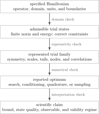
Every arrow is a possible failure point. The upper-bound theorem enters only after the Hamiltonian and admissible domain are fixed; expressivity, optimization, numerical evaluation, and interpretation require additional checks.

Rapid Triage

Symptom	Diagnosis and first response
The objective changes when $\psi$ is rescaled	The normalization denominator is probably missing. Test $c\psi$, then use the Rayleigh quotient or enforce unit norm.
An analytic value lies below a known ground energy	The state may be inadmissible, a surface term may be missing, or the Hamiltonian may differ. Check the form domain and boundaries before recomputing the quadratic form.
Optimization returns a state in the wrong sector	A symmetry or orthogonality constraint is absent. Measure projectors or conserved quantum numbers, then build or project a sector-adapted ansatz.
Energy stabilizes while observables drift	The ansatz may be rigid or the spectral gap small. Enlarge the family and add the missing tail, cusp, correlation, or sector structure.
Different initial parameters give different answers	Expect local minima, flat directions, or poor scaling. Use multiple starts and scaled gradients, then nondimensionalize or reparameterize.
A larger calculation raises the energy	The spaces may not be nested, the searches may be incomplete, or numerics may be unstable. Recompute the old state in the new space and tighten the calculation.
A sampled energy falls slightly below a known bound	A finite-sample fluctuation is possible. Compare the deficit with an autocorrelation-aware uncertainty and validate on fresh samples.
A Ritz value appears to approximate continuum structure	Suspect spectral pollution or box discretization. Vary the box and basis, then use min–max and scattering-aware diagnostics.
Variational and perturbative values disagree at strong coupling	Their validity regimes may not overlap. Identify a shared dimensionless control parameter and compare only where both are controlled.
A time-dependent variational trajectory drifts in energy	Separate manifold-projection error from tangent-solve and time-step errors before changing the ansatz or integrator.

The table locates a starting point, not a verdict. Several failures can coexist, especially in many-parameter or stochastic calculations.

Pitfall 1: Forgetting Normalization

Symptom

The proposed energy depends on the overall amplitude of the trial function, or minimization drives the state toward zero norm.

Mechanism

The numerator alone,

$$N_H[\psi] = \langle\psi\rvert H\lvert\psi\rangle,$$

is not an energy expectation for an arbitrary unnormalized state. Under $\psi\mapsto c\psi$,

$$N_H[c\psi] = \lvert c\rvert^2N_H[\psi].$$

If $N_H[\psi]\gt0$, the numerator can be made arbitrarily small by taking $c\to0$. If it is negative, its magnitude can be made arbitrarily large by rescaling. Neither behavior changes the physical ray represented by the state.

The Rayleigh quotient removes this unphysical direction:

$$\mathcal R_H[c\psi] = \frac{ \lvert c\rvert^2 \langle\psi\rvert H\lvert\psi\rangle }{ \lvert c\rvert^2 \langle\psi\vert\psi\rangle } = \mathcal R_H[\psi].$$

One may instead impose $\lVert\psi\rVert=1$ with a Lagrange multiplier. That is equivalent only when the constraint is actually enforced. Merely writing a multiplier and then optimizing the unconstrained numerator numerically does not remove norm drift.

In a nonorthogonal finite basis,

$$\lvert\psi\rangle = \sum_i c_i\lvert\phi_i\rangle,$$

the norm is $c^\dagger S c$, not $c^\dagger c$, where

$$S_{ij} = \langle\phi_i\vert\phi_j\rangle.$$

Forgetting $S$ changes both the normalization and the stationary equation. The correct Rayleigh–Ritz problem is

$$Hc=ESc.$$

Diagnostic

Perform the rescaling test. Choose several nonzero complex numbers $c$ and verify that the implemented objective is unchanged for $c\psi$. Also check the norm independently by analytic integration, high-accuracy quadrature, or a separate code path.

For normalized parameterizations, monitor

$$\delta_N = \lvert\langle\psi\vert\psi\rangle-1\rvert.$$

A small $\delta_N$ does not establish admissibility, but a large one exposes a normalization failure immediately.

Repair

• Keep the denominator explicit until normalization has been independently verified.
• Remove pure amplitude and phase directions from the parameterization when possible.
• In nonorthogonal bases, use the overlap matrix consistently in norms, gradients, and eigenproblems.
• In Monte Carlo calculations, distinguish normalization-free ratios from an assumption that the sampler already has the intended stationary distribution.

Pitfall 2: Violating Boundary Conditions or the Energy Domain

Symptom

A trial state gives an energy below a rigorous ground-state value, integration by parts produces an unexplained surface term, or the kinetic energy changes depending on which formally equivalent expression is used.

Mechanism

Square integrability is not enough. The trial state must belong to the form domain of the Hamiltonian and obey the boundary conditions that define the self-adjoint problem.

Consider a particle in an infinite well on $0\lt x\lt L$ with Dirichlet conditions. The kinetic quadratic form is

$$q_T[\psi] = \frac{\hbar^2}{2m} \int_0^L \lvert\psi'(x)\rvert^2,dx,$$

with form domain $H_0^1(0,L)$. The normalized constant function

$$\psi_c(x) = \frac{1}{\sqrt L}$$

lies in $L^2(0,L)$ but not in $H_0^1(0,L)$ because it does not vanish at the walls. Applying $-\hbar^2d^2/(2m,dx^2)$ only in the open interval and declaring $\psi_c''=0$ would produce the spurious value zero, below the exact ground energy. The omitted wall discontinuities carry precisely the singular structure that invalidates that calculation.

The same issue appears less dramatically when a radial ansatz is irregular at the origin, a wavefunction has a tail too slow for finite kinetic or potential energy, or a derivative discontinuity is inserted where the differential equation requires another matching condition.

Operator and form domains should not be conflated. A trial state can be admissible for the quadratic form even when $H\psi$ is not a Hilbert-space vector. Conversely, a pointwise formula that looks smooth almost everywhere can fail the form-domain test because of boundaries or singularities. The canonical domain discussion is in Boundary Conditions and Unbounded Operators.

Diagnostic

Check all of the following before optimization:

1. The norm is finite on the physical configuration space.
2. The kinetic and potential quadratic forms are finite.
3. Essential, periodic, Robin, matching, or regularity conditions are satisfied.
4. Every integration by parts has a controlled boundary term.
5. Singular points, particle coincidences, and nodes are treated with the correct local behavior.
6. The numerical discretization imposes the same domain as the stated continuum Hamiltonian.

A useful consistency test is to evaluate the kinetic energy both as a derivative norm and, when justified, as an operator expectation:

$$\frac{\hbar^2}{2m} \int\lvert\nabla\psi\rvert^2,dR \stackrel{?}{=} -\frac{\hbar^2}{2m} \int\psi^*\nabla^2\psi,dR.$$

Disagreement points to boundary, regularity, or numerical differentiation error; equality is valid only under the required domain assumptions.

Repair

Build boundary and regularity conditions into the ansatz rather than asking the optimizer to discover them. Factor out known endpoint powers, cusp factors, angular behavior, or asymptotic decay. If a basis imposes an artificial box or cutoff, report that modified problem and study convergence as the boundary is moved.

Pitfall 3: Ignoring Symmetry and Target-Sector Constraints

Symptom

The optimizer finds a lower state than the one intended, an excited-state search collapses toward the ground state, or observables violate an exact conserved quantum number.

Mechanism

If a projector $P$ commutes with the Hamiltonian,

$$[H,P]=0,$$

then $P\mathcal H$ is an invariant sector. Minimization within that sector bounds its lowest energy,

$$\mathcal R_H[\psi] \geq E_0^{(P)}, \qquad \psi\in P\mathcal H.$$

Without the sector restriction, ordinary minimization seeks the absolute ground state instead. An odd-parity ansatz cannot approximate an even ground state; an unconstrained ansatz intended for the first odd level can simply acquire an even component and lower its energy.

Fermionic exchange symmetry is not optional. A distinguishable-particle product state can have a very low expectation value while being inadmissible for identical fermions. The same warning applies to angular momentum, total spin, lattice momentum, particle number, gauge constraints, and any exact superselection rule relevant to the model.

Broken-symmetry trial states require a more careful statement. They can be useful mean-field coordinates and may describe order in a large system, but a broken-symmetry ansatz is not automatically an eigenstate of the finite-system symmetry. Projection before or after variation defines different approximations and should be named explicitly.

For excited states, orthogonality to approximate lower states is not generally enough to inherit a rigorous upper bound. The correct theorem is the Min–Max Principle, formulated with subspaces and ordered Ritz values.

Diagnostic

• Evaluate $\langle P\rangle$ and, when $P$ is a projector, its leakage $1-\langle P\rangle$.
• Compute $\langle G^2\rangle-\langle G\rangle^2$ for a conserved generator $G$, such as $J_z$, when a definite quantum number is claimed.
• Block the Hamiltonian by exact symmetry before truncation and verify that forbidden matrix elements vanish numerically.
• For an excited-state result, state whether the guarantee comes from exact orthogonality, a min–max subspace, a penalty objective, or only heuristic state following.

Repair

Use symmetry-adapted basis functions, projectors, equivariant parameterizations, or exact constraints. When deliberately breaking a symmetry, report the finite-system symmetry content and compare projected and unprojected energies where meaningful. Never label a penalty-method stationary value a rigorous excited-state upper bound without checking the theorem’s hypotheses.

Pitfall 4: Using an Ansatz That Is Too Rigid

Symptom

The gradient vanishes and the optimizer is reproducible, yet the energy remains poor, residuals remain large, or physically important observables fail to converge.

Mechanism

At a stationary point of a parameterized family $\lvert\psi(\boldsymbol\theta)\rangle$, the residual

$$\lvert r\rangle = (H-E)\lvert\psi\rangle$$

obeys

$$\operatorname{Re} \langle\partial_a\psi\vert r\rangle =0$$

for every available tangent direction. This does not imply $r=0$. It says only that the optimizer cannot lower the energy by moving along the directions represented by the current ansatz.

A one-parameter Gaussian can adjust a length scale but cannot independently repair a cusp, a long-distance tail, nodal topology, and many-body correlation. Adding several parameters of the same ineffective type may leave the missing direction absent.

Rigid and overparameterized are not opposites in a simple sense. A family can contain thousands of redundant coordinates yet still enforce the wrong nodal surface or entanglement pattern. Expressivity concerns the represented states, not the raw parameter count.

Diagnostic

Use structural enlargement rather than parameter-count rhetoric:

1. Compare physically different trial families.
2. Enlarge a genuinely nested linear or nonlinear family.
3. Monitor the residual or energy variance when defined.
4. Track observables sensitive to tails, nodes, contacts, and correlations.
5. Test exact limits and known short- or long-distance behavior.

For nested sets $\mathcal T_1\subseteq\mathcal T_2$,

$$E_{\mathcal T_2} \leq E_{\mathcal T_1}.$$

Failure of this monotonicity means that at least one reported value is not the exact optimum of the stated nested set, or that numerical evaluation has changed. By contrast, two families with more parameters but no set inclusion need not be ordered.

Repair

Add the physics indicated by the diagnostic: the correct asymptotic tail, a cusp factor, another symmetry sector, explicit pair correlation, additional configurations, or a larger entanglement structure. The detailed design principles belong to Trial Wavefunctions and Gaussian Variational Methods.

Pitfall 5: Treating Energy Accuracy as Wavefunction Accuracy

Symptom

Two trial states have nearly identical energies but predict noticeably different radii, densities, response coefficients, transition amplitudes, or entanglement measures.

Mechanism

Energy is stationary at an exact eigenstate. For a normalized state

$$\lvert\psi\rangle = \sqrt{1-\epsilon^2}\,\lvert0\rangle + \epsilon e^{i\phi}\lvert1\rangle,$$

the energy error is quadratic in the contamination:

$$E[\psi]-E_0 = \epsilon^2(E_1-E_0).$$

For an observable $A$, however,

$$\begin{aligned} \langle A\rangle_\psi -\langle A\rangle_0 ={}& 2\epsilon \sqrt{1-\epsilon^2} \operatorname{Re} \left( e^{i\phi}A_{01} \right) \\ &+ \epsilon^2(A_{11}-A_{00}). \end{aligned}$$

When $A_{01}\ne0$, the observable error can be first order in $\epsilon$. The phase $\phi$ can be invisible to the energy yet visible to $A$.

If the ground state is nondegenerate and separated by a known gap $\Delta\gt0$, one can infer

$$1- \lvert\langle0\vert\psi\rangle\rvert^2 \leq \frac{E[\psi]-E_0}{\Delta}.$$

This is useful only when $E_0$ and a usable gap bound are available. A small gap makes the same energy error compatible with much larger state contamination. The full fidelity and observable discussion is in the chapter overview.

Energy variance adds a different test:

$$\sigma_H^2 = \langle(H-E)^2\rangle.$$

Zero variance identifies an energy eigenspace, not necessarily the desired eigenstate. A small variance also needs spectral information before it becomes a quantitative state-distance statement.

Diagnostic

Choose validation observables before optimization. Include quantities with failure mechanisms different from the energy objective:

• short-distance densities or cusp-sensitive observables;
• long-distance radii and tail probabilities;
• symmetry projectors and conserved quantities;
• transition or response matrix elements;
• residual norms or local-energy variance;
• overlap with a benchmark state when one exists.

Report whether each observable was used to fit the ansatz. Agreement on a fitted quantity is weaker evidence than a successful out-of-sample prediction.

Repair

Do not replace the energy objective casually; add diagnostics and enlarge the state family in the directions those diagnostics expose. When the scientific target is a particular observable, establish its own convergence and uncertainty budget. For unbounded observables, an energy estimate alone generally supplies no uniform error bound.

Pitfall 6: Optimizing Without Checking Units and Scales

Symptom

An optimizer zigzags, takes vanishingly small steps, pushes positive widths through zero, reports incompatible gradient magnitudes, or converges to different answers after a change of units.

Mechanism

Coordinate gradients inherit the units and arbitrary scaling of their parameters. If $a$ is an inverse length and $b$ is a length squared, the raw numbers $\partial E/\partial a$ and $\partial E/\partial b$ cannot be compared as though they were components in an orthonormal Euclidean space.

Nondimensionalization should precede numerical optimization. Choose characteristic scales $L_\star$ and $E_\star$, then write

$$x=L_\star y, \qquad H=E_\star\widetilde H, \qquad \theta^a=\theta_\star^a u^a.$$

The dimensionless objective

$$\widetilde E(\mathbf u) = \frac{E(\boldsymbol\theta)}{E_\star}$$

has gradients that can be interpreted on a common scale. Positive parameters spanning orders of magnitude are often better represented by

$$u^a = \log \left( \frac{\theta^a}{\theta_\star^a} \right).$$

Poor scaling can coexist with genuine coordinate redundancy. Nearly identical basis vectors make the overlap matrix ill-conditioned; gauge directions or normalization parameters can make the state-space metric singular. Blindly inverting a Hessian, overlap matrix, or metric then amplifies numerical error.

Diagnostic

Before trusting the final energy:

1. Nondimensionalize the Hamiltonian and parameters.
2. Compare analytic or automatic gradients with finite differences over several step sizes.
3. Use multiple physically distinct starting points.
4. Report a scaled gradient or projected residual, not only successive energy changes.
5. Inspect Hessian, overlap, or state-metric eigenvalues.
6. Vary integration tolerance, basis threshold, damping, and trust radius.
7. Re-evaluate the final state with a tighter and preferably independent evaluator.

A stationary point must also be classified. In one parameter, $dE/d\theta=0$ can be a minimum, maximum, or inflection point. In many parameters, negative Hessian directions expose saddles. Boundary minima require constrained optimality conditions rather than an unconstrained zero gradient.

The numerical details and geometry-aware updates are developed in Variational Parameters and Conditioning and Stability.

Repair

Use natural units, logarithmic positive coordinates, orthogonalized bases, rank-revealing factorizations, damping, line searches, or trust regions as appropriate. A sophisticated optimizer cannot repair an incorrect objective or an inexpressive ansatz, so optimization improvements should be paired with independent state diagnostics.

Pitfall 7: Comparing Variational and Perturbative Results Outside a Common Regime

Symptom

A variational upper bound and a truncated perturbation series disagree, and the disagreement is presented as proof that one method is wrong even though their validity assumptions do not overlap.

Mechanism

The methods certify different things. An exact variational expectation is an upper bound for an admissible state. A truncated perturbation series is generally neither an upper nor a lower bound. Perturbation theory is controlled by a small dimensionless parameter and can be highly accurate within that regime; a variational family can remain finite outside it but may carry uncontrolled ansatz bias.

The quartic oscillator makes the distinction explicit. In units $\hbar=m=\omega=1$, let

$$H = \frac{p^2}{2} + \frac{x^2}{2} + g x^4, \qquad g\geq0.$$

For the normalized Gaussian

$$\psi_a(x) = \left( \frac{a}{\pi} \right)^{1/4} e^{-a x^2/2}, \qquad a\gt0,$$

the exact Rayleigh quotient within this family is

$$E_{\mathrm G}(a) = \frac{a}{4} + \frac{1}{4a} + \frac{3g}{4a^2}.$$

Stationarity gives

$$a^3-a-6g=0.$$

At weak coupling,

$$a_\star = 1+3g+O(g^2),$$

and therefore

$$E_{\mathrm G}(a_\star) = \frac{1}{2} + \frac{3}{4}g + O(g^2).$$

The coefficient $3/4$ agrees with first-order perturbation theory because both methods are being compared in their common small-$g$ regime. At strong coupling, the Gaussian optimum instead has

$$a_\star \sim (6g)^{1/3},$$

so

$$E_{\mathrm G}(a_\star) \sim \frac{3}{8} (6g)^{1/3}.$$

The first-order perturbative expression grows linearly with $g$ and is not a controlled strong-coupling approximation. Its disagreement with the variational scaling is expected, not paradoxical. The Gaussian value remains an upper bound, but the bound alone does not quantify its strong-coupling error.

Diagnostic

For each method, write down:

• its dimensionless control parameter;
• the observable and Hamiltonian being approximated;
• the retained order or trial family;
• the regime in which omitted terms are expected to be small;
• whether the output carries a one-sided bound, an asymptotic estimate, or no formal error sign.

Only compare accuracy claims where these regimes overlap. Matching the leading weak-coupling expansion of a variational result is a valuable internal check; agreement at one fitted parameter value is much weaker.

Repair

Use perturbative information to design or test the ansatz, and use variational calculations as nonperturbative benchmarks only with an explicit ansatz-convergence study. When one method must interpolate between regimes, Variational Perturbation Theory provides a controlled vocabulary for order-dependent reorganizations; it does not turn every truncated expression into a rigorous bound.

Related Failures That Look Like Theorem Violations

The reported number is not the exact quotient

Suppose an admissible state has exact energy $E(\theta)$, but a calculation reports

$$\widehat E = E(\theta) + \delta_{\mathrm{quad}} + \delta_{\mathrm{basis}} + \delta_{\mathrm{stat}} + \delta_{\mathrm{impl}}.$$

Quadrature, derivative discretization, basis-conditioning error, finite-sample noise, and implementation mistakes need not have a positive sign. Thus $\widehat E\lt E_0$ does not logically refute the variational principle. It is a diagnostic that the evaluation and uncertainty budget must be examined.

In Variational Monte Carlo, a finite-sample mean can fall below $E_0$ by chance. Autocorrelation, equilibration, heavy-tailed local energies, reuse of optimization samples, and estimator bias all affect the interpretation. The final energy should be validated on fresh samples with an autocorrelation-aware uncertainty.

The Hamiltonian changed

Replacing $H$ by a projected, discretized, pseudopotential, finite-volume, or effective Hamiltonian $H_{\mathrm{eff}}$ changes the theorem’s target. The exact statement is then

$$\mathcal R_{H_{\mathrm{eff}}}[\psi] \geq \inf\sigma(H_{\mathrm{eff}}),$$

not necessarily a bound on $\inf\sigma(H)$. A result can converge perfectly for the wrong model. Report model error separately from trial-space and numerical error.

More basis functions did not produce a lower value

Monotone variational improvement requires exact optimization over nested spaces using consistent matrix elements. If an energy rises after increasing a cutoff, ask:

1. Is the old space exactly contained in the new one?
2. Can the old optimized state be represented and re-evaluated in the new calculation?
3. Did nonlinear basis parameters change both spaces?
4. Did an overlap threshold discard a different subspace?
5. Were both optimization problems solved to comparable tolerances?

An increase is useful evidence about the implementation or comparison protocol; it is not mysterious behavior permitted by the variational theorem.

A time-dependent variational principle was treated as static minimization

The Time-Dependent Variational Principle chooses a tangent-space motion that makes an action stationary or a dynamical residual small. It does not generally minimize the instantaneous energy. Energy drift can arise from the restricted manifold, an approximate tangent solve, or the time integrator. Those errors must be separated before changing the static ansatz.

False Successes

Some failures produce reassuring numbers.

Agreement between dependent calculations

Two codes can agree because they share the same basis, pseudopotential, boundary condition, quadrature, or convention error. Prefer benchmarks with different failure mechanisms: analytic limits, exact diagonalization in a smaller system, independent trial families, residual identities, or known inequalities.

A stable decimal without a convergence parameter

Optimizer iterations can stabilize while ansatz error remains unchanged. Every numerical stability claim should name the parameter that was varied: basis size, domain size, quadrature order, sample count, time step, rank threshold, or optimizer tolerance.

A very low energy from a highly flexible ansatz

Lower is better only for exact expectations of the same Hamiltonian over admissible states. With noisy training data, a flexible ansatz can exploit estimator fluctuations; with an ill-conditioned basis, it can exploit roundoff; with a modified loss, it can optimize something other than energy. Re-evaluate the frozen state independently.

Zero variance without state identification

Every exact energy eigenstate has zero energy variance. A zero-variance state may be an excited state or lie in a degenerate eigenspace. Use energy, symmetry, and overlap information to identify the state.

A Verification Protocol

Before treating a variational result as mature, record the following ledger.

1. Model: Hamiltonian, domain, boundary conditions, units, cutoffs, and effective approximations.
2. Target: ground state, symmetry-sector minimum, ordered Ritz level, or dynamical trajectory.
3. Trial class: analytic form, basis, parameter constraints, symmetry, asymptotics, and nesting relation.
4. Objective: exact quotient, penalized loss, stochastic estimator, projected Hamiltonian, or another quantity.
5. Optimization: starts, stopping test, scaled gradient, curvature or metric conditioning, and constraint handling.
6. Evaluation: quadrature or sample error, rank thresholds, derivative checks, and independent re-evaluation.
7. State diagnostics: residual or variance, symmetry leakage, limiting behavior, and relevant observables.
8. Convergence: systematic enlargement or comparison with an independently biased family.
9. Claim: exactly which bound, approximation, uncertainty, and validity regime is supported.

This protocol is deliberately redundant. A result becomes trustworthy when several independent checks fail in different ways and nevertheless converge on the same conclusion.

Exercises

1. Why the numerator alone collapses

Let $H$ be positive and let $\psi$ be a nonzero state with finite energy. Show that minimizing $\langle\psi\rvert H\lvert\psi\rangle$ over unconstrained scalar multiples of $\psi$ has infimum zero. Explain why this says nothing about the ground-state energy.

Solution

For $c\ne0$,

$$\langle c\psi\rvert H\lvert c\psi\rangle = \lvert c\rvert^2 \langle\psi\rvert H\lvert\psi\rangle.$$

Taking $c\to0$ makes the numerator approach zero. The physical ray has not changed; only its representative’s norm has. The ground-state variational problem fixes the norm or divides by it, so that this unphysical rescaling cannot lower the objective.

2. The constant function in an infinite well

On $0\lt x\lt L$, explain why the normalized constant function cannot be used to claim a zero variational energy for an infinite square well. Which hypothesis fails?

Solution

The infinite-well Hamiltonian has Dirichlet boundary conditions. Its kinetic form domain is $H_0^1(0,L)$, whose elements have vanishing boundary trace. The constant function does not vanish at $x=0$ or $x=L$, so it is not admissible even though it is square-integrable.

Treating its second derivative as zero only inside the open interval ignores the discontinuity required to join it to the vanishing exterior. The variational theorem therefore does not apply to this trial function for that Hamiltonian.

3. Sector targeting

Let $P$ be an orthogonal projector with $[H,P]=0$. A normalized trial state has sector weight $p=\langle P\rangle$ with $0\lt p\lt1$. Why does minimizing its total energy not necessarily approximate the lowest state in $P\mathcal H$? Give a direct repair.

Solution

Write

$$\lvert\psi\rangle = \sqrt p\,\lvert\psi_P\rangle + \sqrt{1-p}\,\lvert\psi_\perp\rangle,$$

with normalized components in the two invariant sectors. Because $[H,P]=0$, cross terms vanish and

$$E[\psi] = pE[\psi_P] + (1-p)E[\psi_\perp].$$

If the complementary sector has a lower energy, unconstrained minimization can lower the objective by reducing $p$. It then targets the wrong sector. One repair is to parameterize states entirely inside $P\mathcal H$; another is to project and normalize,

$$\lvert\widetilde\psi_P\rangle = \frac{P\lvert\psi\rangle}{\sqrt{\langle P\rangle}},$$

provided $p\ne0$.

4. Stationarity inside a rigid family

Let $H\lvert n\rangle=E_n\lvert n\rangle$ with $E_0\lt E_1\lt E_2$, and consider

$$\lvert\psi(\theta)\rangle = \cos\theta\lvert1\rangle + \sin\theta\lvert2\rangle.$$

Find the minimum over this family. Why does exact optimization still fail to approximate the ground state?

Solution

The energy is

$$E(\theta) = E_1\cos^2\theta + E_2\sin^2\theta.$$

Because $E_2\gt E_1$, the minimum occurs at $\theta=0$ modulo $\pi$, with value $E_1$. The optimization is exact inside the family, but the family is orthogonal to $\lvert0\rangle$ and cannot represent the ground state. A vanishing parameter gradient diagnoses stationarity only within the represented tangent direction.

5. Energy and observable sensitivity

For

$$\lvert\psi\rangle = \sqrt{1-\epsilon^2}\,\lvert0\rangle + \epsilon\lvert1\rangle,$$

take $A=\lvert0\rangle\langle1\rvert+\lvert1\rangle\langle0\rvert$. Compute the energy error and $\langle A\rangle_\psi$. Compare their leading powers in $\epsilon$.

Solution

The energy is diagonal in its eigenbasis, so

$$E[\psi]-E_0 = \epsilon^2(E_1-E_0).$$

The observable interchanges the two states, giving

$$\langle A\rangle_\psi = 2\epsilon\sqrt{1-\epsilon^2} = 2\epsilon+O(\epsilon^3).$$

Thus the energy error is quadratic while this observable error is linear. An apparently excellent energy can coexist with a more visible error in an off-diagonal observable.

6. Weak- and strong-coupling checks for the quartic oscillator

Starting from

$$E_{\mathrm G}(a) = \frac{a}{4} + \frac{1}{4a} + \frac{3g}{4a^2},$$

derive the stationarity equation. Then obtain the leading weak-$g$ correction to $a$ and the strong-$g$ energy scaling.

Solution

Differentiation gives

$$\frac{dE_{\mathrm G}}{da} = \frac14 - \frac{1}{4a^2} - \frac{3g}{2a^3}.$$

Multiplying the stationary equation by $4a^3$ yields

$$a^3-a-6g=0.$$

For weak coupling, write $a=1+cg+O(g^2)$. Then

$$a^3-a-6g = (2c-6)g+O(g^2),$$

so $c=3$. Because the unperturbed energy is already stationary at $a=1$, the $O(g)$ width change does not alter the harmonic part at first order, and

$$E_{\mathrm G} = \frac{1}{2} + \frac{3}{4}g + O(g^2).$$

For $g\to\infty$, the stationarity equation gives $a^3\sim6g$. The harmonic-potential term $1/(4a)$ is subleading, while

$$\frac{3g}{4a^2} \sim \frac{a}{8}.$$

Therefore

$$E_{\mathrm G} \sim \frac{3a}{8} \sim \frac38(6g)^{1/3}.$$

7. Diagnosing a nonmonotone basis result

A calculation reports $E_N=-1.24$ in an $N$-dimensional space and $E_{N+1}=-1.22$ after adding one basis vector. List three logically distinct explanations consistent with the variational principle.

Solution

Possible explanations include:

1. The two spaces are not actually nested, perhaps because nonlinear basis parameters or an orthogonalization threshold changed.
2. One or both optimizations are incomplete, so the reported values are not the exact minima in their spaces.
3. Matrix elements, overlap conditioning, quadrature, or rounding errors changed the evaluated objective.

If the spaces are nested and evaluated consistently, the old optimized vector remains available in the larger space. Its re-evaluated energy supplies an immediate upper bound on the new optimum, so an exact larger-space minimum cannot be higher.

References

1. W. Ritz, “Über eine neue Methode zur Lösung gewisser Variationsprobleme der mathematischen Physik”, Journal für die reine und angewandte Mathematik 135, 1–61 (1909). Foundational Rayleigh–Ritz construction.
2. J. K. L. MacDonald, “Successive Approximations by the Rayleigh–Ritz Variation Method”, Physical Review 43, 830–833 (1933). Classic discussion of successive variational eigenvalue approximations.
3. T. Kato, Perturbation Theory for Linear Operators, 2nd ed. (Springer, 1995). Standard source for self-adjoint operators, closed forms, domains, and spectral approximation.
4. M. Reed and B. Simon, Methods of Modern Mathematical Physics, Vol. IV: Analysis of Operators (Academic Press, 1978). Spectral and min–max foundations for Schrödinger operators.
5. R. K. Nesbet, Variational Principles and Methods in Theoretical Physics and Chemistry (Cambridge University Press, 2003). Broad graduate treatment of static and time-dependent variational methods.
6. J. Nocedal and S. J. Wright, Numerical Optimization, 2nd ed. (Springer, 2006). Optimization diagnostics, scaling, constraints, line searches, and trust regions.
7. A. Szabo and N. S. Ostlund, Modern Quantum Chemistry: Introduction to Advanced Electronic Structure Theory (Dover, 1996). Variational basis methods, symmetry, and nonorthogonal orbital calculations.
8. W. M. C. Foulkes, L. Mitas, R. J. Needs, and G. Rajagopal, “Quantum Monte Carlo simulations of solids”, Reviews of Modern Physics 73, 33–83 (2001). Variational Monte Carlo, trial-state bias, optimization, and statistical diagnostics.