Gauge, Phase, and Magnetic Geometry

Quantum mechanics is a theory of amplitudes, so phase is part of its basic structure. One overall phase does not change a pure state ray, but relative phases control interference. When the phase convention is allowed to vary from point to point, ordinary derivatives are no longer covariant. A connection is then needed to compare phases at neighboring points.

In nonrelativistic electromagnetic quantum mechanics, the scalar and vector potentials supply that connection. Their local curvature gives the electric and magnetic fields, while their transport around closed loops gives gauge-invariant holonomy. This one structure explains:

• the replacement $\mathbf p\mapsto\mathbf p-q\mathbf A$;
• the Aharonov–Bohm phase around excluded flux;
• the noncommuting algebra of magnetic translations;
• the guiding-center degeneracy of Landau levels;
• the need for gauge patches around a Dirac monopole;
• the Peierls phase on lattice links.

The chapter is deliberately scoped. It treats prescribed electromagnetic backgrounds and $U(1)$ phase geometry inside nonrelativistic quantum mechanics. Quantized gauge fields, photons, nonabelian gauge dynamics, renormalization, and the full field-theoretic meaning of local gauge redundancy belong to later QFT material.

Canonical Boundaries

This page owns the chapter map and the common geometric logic. Detailed derivations and application-specific calculations remain at their canonical homes.

Topic	Canonical home	Role here
ray phase freedom	Global Phase and Physical States	separates global phase redundancy from observable relative phase
position-dependent phase	Local Phase Transformations	derives why ordinary derivatives fail and covariant derivatives are needed
electromagnetic coupling rule	Minimal Coupling	interprets $\boldsymbol\pi=\mathbf p-q\mathbf A$ and its commutators
equivalence of representatives	Gauge Transformations in Quantum Mechanics	owns the complete $\psi$, $\mathbf A$, $\Phi$ transformation and observable checklist
translation algebra in a field	Magnetic Translations	derives the flux-dependent projective group law
loop phase around excluded flux	Aharonov–Bohm Effect	owns the real-space holonomy and topology interpretation
patching and magnetic charge	Dirac Monopole Preview	derives the two-patch quantization argument and Berry-monopole analogy
uniform-field symmetry structure	Landau Levels Revisited	separates cyclotron energy from guiding-center degeneracy
lattice link transport	Peierls Phase Preview	connects continuum gauge covariance to tight-binding hopping phases

The coordinate-space solution of charged-particle systems belongs to Electromagnetic Fields. Berry connections over parameter space begin with Geometric Phases and Topology. The bridge from this $U(1)$ wave-mechanics structure to dynamical gauge theory is From Phase Symmetry to Gauge Theory.

The Organizing Pattern

The chapter follows one hierarchy:

$$\begin{gathered} \text{phase representative} \\ \longrightarrow \\ \text{connection} \\ \longrightarrow \\ \text{curvature} \\ \longrightarrow \\ \text{holonomy} \\ \longrightarrow \\ \text{observable interference}. \end{gathered}$$

A connection tells how to compare phases at neighboring points. Curvature measures the failure of infinitesimal transports to commute. Holonomy records the result of transport around a finite closed loop.

In electromagnetic wave mechanics:

Geometric role	Electromagnetic object
local phase representative	$\psi(\mathbf r,t)$
connection data	$(\Phi,\mathbf A)$
curvature data	$(\mathbf E,\mathbf B)$
loop holonomy	$\exp[(iq/\hbar)\oint\mathbf A\cdot d\mathbf r]$

The potentials are gauge dependent, the fields are gauge invariant, and the closed-loop phase is gauge invariant under allowed transformations. These are different levels of the same geometry.

Global Phase and the Ray

A nonzero vector and any nonzero scalar multiple define the same pure-state ray:

$$|\psi\rangle \sim \lambda|\psi\rangle, \qquad \lambda\in\mathbb C\setminus\{0\}.$$

After normalization, the remaining freedom is

$$|\psi\rangle \sim e^{i\alpha}|\psi\rangle.$$

The rank-one projector

$$\Pi_\psi = |\psi\rangle\langle\psi|$$

is unchanged by this transformation:

$$e^{i\alpha} |\psi\rangle\langle\psi| e^{-i\alpha} = \Pi_\psi.$$

Probabilities and expectation values therefore do not depend on the overall phase of a single state representative.

This does not make every phase unphysical. For

$$|\psi\rangle = \frac{1}{\sqrt2} \left( |0\rangle +e^{i\varphi}|1\rangle \right),$$

$\varphi$ is a relative phase. It changes interference observables and cannot be removed by multiplying the entire state by one number.

The useful statement is:

One global phase of one isolated state vector is redundant; phase differences between coherent alternatives are observable.

This distinction is what lets a closed-loop phase become measurable in an interferometer. One branch acquires the phase while another supplies the reference.

Phase Conventions over a Family

Suppose normalized states depend smoothly on parameters $R$. Choosing one vector $|\psi(R)\rangle$ on each ray is a local phase gauge:

$$|\psi(R)\rangle \mapsto e^{i\chi(R)} |\psi(R)\rangle.$$

With the Berry-connection convention

$$\mathcal A(R) = i\langle\psi(R)| \nabla_R\psi(R)\rangle,$$

the phase change gives

$$\mathcal A(R) \mapsto \mathcal A(R) -\nabla_R\chi(R).$$

The connection is gauge dependent. Its curvature and closed-loop holonomy provide gauge-invariant information.

The symbol and sign here belong to a parameter-space Berry convention. The electromagnetic convention below uses $\mathbf A\mapsto\mathbf A+\nabla\chi$ together with $\psi\mapsto e^{iq\chi/\hbar}\psi$. The two structures are analogous, but their symbols and sign conventions should not be mixed without checking definitions.

From Global to Local Phase

For a charged wavefunction, consider

$$\psi'(\mathbf r,t) = e^{iq\chi(\mathbf r,t)/\hbar} \psi(\mathbf r,t).$$

The density is unchanged:

$$|\psi'|^2=|\psi|^2.$$

But a derivative detects the position dependence:

$$\begin{aligned} \nabla\psi' &= e^{iq\chi/\hbar} \nabla\psi \\ &\quad+ e^{iq\chi/\hbar} \frac{iq}{\hbar} (\nabla\chi)\psi . \end{aligned}$$

The extra term vanishes for a constant phase but not for a local one. A derivative compares values at neighboring points; it therefore needs a rule for aligning their phase conventions.

The canonical momentum

$$\mathbf p=-i\hbar\nabla$$

accordingly transforms as

$$\mathbf p\psi' = e^{iq\chi/\hbar} \left[ \mathbf p\psi +q(\nabla\chi)\psi \right].$$

Canonical momentum acting by itself is not gauge covariant.

Covariant Derivatives and Minimal Coupling

Introduce

$$D_i = \partial_i -\frac{iq}{\hbar}A_i,$$

and transform

$$\mathbf A' = \mathbf A+\nabla\chi.$$

Then

$$D_i'\psi' = e^{iq\chi/\hbar} D_i\psi.$$

The covariant derivative transforms in the same way as the wavefunction. The corresponding kinetic momentum is

$$\boldsymbol\pi = -i\hbar\mathbf D = \mathbf p-q\mathbf A.$$

It obeys

$$\boldsymbol\pi'\psi' = e^{iq\chi/\hbar} \boldsymbol\pi\psi.$$

Minimal coupling is the replacement

$$\mathbf p \longmapsto \boldsymbol\pi = \mathbf p-q\mathbf A.$$

For a spinless particle in prescribed electromagnetic potentials,

$$\begin{aligned} H &= \frac{1}{2m} \left[ \mathbf p -q\mathbf A(\mathbf r,t) \right]^2 \\ &\quad+ q\Phi(\mathbf r,t). \end{aligned}$$

The time component is made covariant with

$$D_t = \partial_t +\frac{iq}{\hbar}\Phi,$$

and

$$\Phi' = \Phi-\partial_t\chi.$$

Then

$$D_t'\psi' = e^{iq\chi/\hbar} D_t\psi,$$

so the Schrödinger equation can be written

$$i\hbar D_t\psi = -\frac{\hbar^2}{2m} \sum_iD_iD_i\psi.$$

Every term transforms covariantly.

Canonical and Kinetic Momentum

Canonical momentum and kinetic momentum should not be used interchangeably.

Quantity	Definition	Physical role
canonical momentum	$\mathbf p=-i\hbar\nabla$	generator tied to a chosen position-space phase convention
kinetic momentum	$\boldsymbol\pi=\mathbf p-q\mathbf A$	mechanical momentum $m\mathbf v$ and gauge-covariant observable

Their elementary commutators are

$$[r_i,\pi_j] = i\hbar\delta_{ij},$$

and

$$[\pi_i,\pi_j] = i\hbar q \sum_k \epsilon_{ijk}B_k.$$

The first preserves the usual position–momentum pairing. The second says that kinetic-momentum components fail to commute in a magnetic field. That noncommutativity is the algebraic seed of Landau quantization.

The velocity operator is

$$\mathbf v = \frac{\boldsymbol\pi}{m}$$

for the scalar minimal-coupling Hamiltonian. Canonical momentum labels can still be useful in a chosen gauge, but they are not generally gauge-invariant mechanical momenta.

Gauge Transformations Relate Equivalent Descriptions

The complete electromagnetic gauge transformation is

$$\begin{aligned} \psi' &= e^{iq\chi/\hbar}\psi, \\ \mathbf A' &= \mathbf A+\nabla\chi, \\ \Phi' &= \Phi-\partial_t\chi. \end{aligned}$$

The triples

$$(\psi,\mathbf A,\Phi) \quad\hbox{and}\quad (\psi',\mathbf A',\Phi')$$

represent the same physical situation when boundary conditions and allowed gauge functions are treated consistently.

Gauge redundancy differs from an ordinary physical symmetry. A spatial translation may move a wavepacket to a physically distinct location. A gauge transformation changes the representative used to describe the same charged-particle configuration.

This does not make the potentials dispensable. Connections are precisely the objects needed to compare local phases. Their individual values depend on gauge, while their curvature and holonomy contain invariant information.

Time-dependent Hamiltonian law

Let

$$U_\chi(\mathbf r,t) = e^{iq\chi(\mathbf r,t)/\hbar}.$$

For a time-dependent gauge transformation,

$$\begin{aligned} H[\mathbf A',\Phi'] &= U_\chi H[\mathbf A,\Phi] U_\chi^\dagger \\ &\quad+ i\hbar (\partial_tU_\chi) U_\chi^\dagger. \end{aligned}$$

The derivative term is essential. Omitting it gives the wrong scalar-potential transformation and breaks covariance of the time-dependent Schrödinger equation.

Gauge-Invariant and Gauge-Covariant Quantities

A quantity is gauge invariant when its numerical value is unchanged. A quantity is gauge covariant when it changes in a controlled way that preserves physical predictions.

Examples:

Quantity	Behavior
$\psi$	covariant: acquires a local phase
$D_\mu\psi$	covariant: acquires the same local phase
$\mathbf A$, $\Phi$	gauge dependent connection representatives
$\rho=	\psi
$\mathbf E$, $\mathbf B$	invariant
gauge-covariant current	invariant
closed-loop phase factor	invariant

The probability current is

$$\mathbf j = \frac{1}{m} \operatorname{Re} \left[ \psi^* \left( -i\hbar\nabla-q\mathbf A \right) \psi \right].$$

Because $\boldsymbol\pi\psi$ transforms with the same phase as $\psi$, the current is gauge invariant.

In polar form,

$$\psi=Re^{iS/\hbar},$$

the local phase transformation gives

$$S\mapsto S+q\chi.$$

The invariant mechanical combination is

$$\nabla S-q\mathbf A,$$

not either term separately.

Connection, Curvature, and Fields

The electromagnetic fields are

$$\mathbf B = \nabla\times\mathbf A,$$

and

$$\mathbf E = -\nabla\Phi -\partial_t\mathbf A.$$

Under the full gauge transformation, both remain unchanged. In geometric language, $(\Phi,\mathbf A)$ are connection data and $(\mathbf E,\mathbf B)$ are curvature data.

Locally, curvature controls force and infinitesimal transport. Globally, a connection can have nontrivial holonomy even in an accessible region where the local curvature vanishes.

For a closed spatial loop $C$, define

$$W(C) = \exp \left[ \frac{iq}{\hbar} \oint_C \mathbf A\cdot d\mathbf r \right].$$

For a smooth single-valued $\chi$,

$$\oint_C \nabla\chi\cdot d\mathbf r =0,$$

so $W(C)$ is gauge invariant. On multiply connected spaces, large gauge transformations and winding require attention, but the exponential remains the invariant object.

Pure Gauge Does Not Always Mean Globally Trivial

If

$$\mathbf A=\nabla\chi, \qquad \Phi=-\partial_t\chi,$$

then

$$\mathbf E=\mathbf0, \qquad \mathbf B=\mathbf0.$$

On a simply connected region with a single-valued $\chi$, the potentials can be removed globally by a gauge transformation.

On a multiply connected region, a connection can be locally pure gauge while retaining nontrivial loop holonomy:

$$\oint_C \mathbf A\cdot d\mathbf r \ne0.$$

The phrase field-free is therefore local. It does not by itself imply that every global phase around a noncontractible loop is trivial.

Aharonov–Bohm Holonomy

The magnetic Aharonov–Bohm setup excludes a flux-carrying region from the particle’s configuration space. Along the accessible paths,

$$\mathbf B=\mathbf0,$$

but a loop winding around the excluded region can satisfy

$$\oint_C \mathbf A\cdot d\mathbf r = \Phi_B.$$

The relative phase of two paths is

$$\Delta\varphi_{\mathrm{AB}} = \frac{q\Phi_B}{\hbar} \quad \operatorname{mod}2\pi.$$

The gauge-invariant statement is the phase factor

$$\exp \left( \frac{iq\Phi_B}{\hbar} \right).$$

The interference is periodic under one flux quantum:

$$\Phi_B \mapsto \Phi_B+\Phi_0, \qquad \Phi_0 = \frac{h}{|q|}.$$

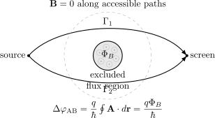
The two accessible paths can be locally field free while their closed combination encloses magnetic flux. The observable is the relative holonomy $\Delta\varphi_{\mathrm{AB}}=(q/\hbar)\oint\mathbf A\cdot d\mathbf r$.

The topology matters because a winding loop cannot be contracted to a point without crossing the excluded region. Stokes’ theorem has not failed: a spanning disk either leaves the accessible space or crosses the flux-carrying core.

The effect does not make the value of $\mathbf A$ at one point observable. It makes the closed-loop holonomy observable through interference.

Magnetic Translations

A uniform magnetic field is physically translation invariant, but a chosen vector potential need not be. Ordinary translations can therefore fail to commute with a gauge-fixed Hamiltonian even when the field is uniform.

Magnetic translations combine a spatial shift with the phase transport required by the connection. For displacement $\mathbf a$, a path-based form is

$$\begin{aligned} (\mathsf T_B(\mathbf a)\psi)(\mathbf r) &= \exp \left[ \frac{iq}{\hbar} \int_{\mathbf r-\mathbf a}^{\mathbf r} \mathbf A\cdot d\boldsymbol\ell \right] \\ &\quad\times \psi(\mathbf r-\mathbf a). \end{aligned}$$

The operation is gauge covariant. In a uniform field it can be chosen to commute with the Landau Hamiltonian.

The striking result is the group law:

$$\begin{aligned} \mathsf T_B(\mathbf a) \mathsf T_B(\mathbf b) &= \exp \left[ \frac{iqB}{\hbar} A(\mathbf a,\mathbf b) \right] \\ &\quad\times \mathsf T_B(\mathbf b) \mathsf T_B(\mathbf a), \end{aligned}$$

where

$$A(\mathbf a,\mathbf b) = a_xb_y-a_yb_x$$

is the signed parallelogram area for $\mathbf B=B\hat{\mathbf z}$.

The phase is

$$\frac{q\Phi_{\mathbf a,\mathbf b}}{\hbar}, \qquad \Phi_{\mathbf a,\mathbf b} = BA(\mathbf a,\mathbf b).$$

Magnetic translations form a projective representation of ordinary translations. Their commutator is a finite-loop Aharonov–Bohm phase.

Landau Levels: Two Noncommutative Planes

For a spinless particle in a uniform perpendicular field,

$$H = \frac{\pi_x^2+\pi_y^2}{2m},$$

with

$$[\pi_x,\pi_y] = i\hbar qB.$$

The kinetic momenta form a cyclotron oscillator and determine

$$E_n = \hbar\omega_c \left( n+\frac12 \right), \qquad \omega_c = \frac{|q|B}{m}.$$

The guiding-center coordinates

$$X = x+\frac{\pi_y}{qB}, \qquad Y = y-\frac{\pi_x}{qB}$$

commute with the Hamiltonian:

$$[X,H]=[Y,H]=0.$$

They do not commute with each other:

$$[X,Y] = -\frac{i\hbar}{qB}.$$

This gives two independent structures:

Plane	Algebraic role	Physical output
cyclotron $(\pi_x,\pi_y)$	oscillator pair	Landau energy ladder
guiding center $(X,Y)$	commuting with $H$ but noncommuting mutually	degeneracy within each level

For a large region of area $\mathcal A$,

$$N_\Phi \approx \frac{|q|B\mathcal A}{h} = \frac{\Phi}{\Phi_0}.$$

Each spinless Landau level has approximately one guiding-center state per flux quantum. Boundaries, spin, disorder, and interactions modify the finite-system bookkeeping but not the origin of the ideal bulk count.

Landau gauge and symmetric gauge organize the same Hilbert space differently. Gauge-dependent labels such as $k_y$ should not be mistaken for universal mechanical momenta.

Global Consistency on a Torus

On a torus with fundamental cycles $\mathbf L_1$ and $\mathbf L_2$, large magnetic translations obey

$$\begin{aligned} \mathsf T_B(\mathbf L_1) \mathsf T_B(\mathbf L_2) &= \exp \left( \frac{iq\Phi_{\mathrm{tot}}}{\hbar} \right) \\ &\quad\times \mathsf T_B(\mathbf L_2) \mathsf T_B(\mathbf L_1). \end{aligned}$$

Ordinary periodic consistency requires

$$\frac{q\Phi_{\mathrm{tot}}}{\hbar} \in 2\pi\mathbb Z.$$

Equivalently, the total flux is an integer number of single-particle flux quanta in magnitude. This is a global boundary-condition statement, not a local equation of motion.

Dirac Monopole and Gauge Patches

A monopole field is

$$\mathbf B(\mathbf r) = g\frac{\mathbf r}{r^3}, \qquad r>0.$$

Its flux through a surrounding sphere is

$$\int_{S^2} \mathbf B\cdot d\mathbf S = 4\pi g.$$

One globally smooth vector potential on that sphere cannot produce nonzero flux. The correct description uses northern and southern patches:

$$A_N = g(1-\cos\theta)d\phi,$$

and

$$A_S = -g(1+\cos\theta)d\phi.$$

On their overlap,

$$A_N-A_S = d(2g\phi).$$

A charge-$q$ wavefunction is patched by

$$\psi_N = \exp \left( \frac{i2qg\phi}{\hbar} \right) \psi_S.$$

Single-valuedness as $\phi\mapsto\phi+2\pi$ requires

$$\exp \left( \frac{i4\pi qg}{\hbar} \right) =1.$$

Therefore

$$2qg=n\hbar, \qquad n\in\mathbb Z$$

in the convention $\mathbf B=g\mathbf r/r^3$.

The convention-independent form is

$$\frac{q}{2\pi\hbar} \int_{S^2} \mathbf B\cdot d\mathbf S \in \mathbb Z.$$

This integer is the first Chern number of the associated $U(1)$ line bundle. The Dirac argument does not prove monopoles exist; it states the consistency condition that follows if they do.

The Berry monopole analogy lives in parameter space rather than physical space. Both use connections, curvature, gauge patches, and quantized flux, but only the Dirac monopole here is an electromagnetic source.

Peierls Phase on a Lattice

In a tight-binding model, continuum phase transport becomes a phase on each hopping link:

$$t_{ij} \longmapsto t_{ij}e^{i\theta_{ij}},$$

with

$$\theta_{ij} = \frac{q}{\hbar} \int_{\mathbf r_j}^{\mathbf r_i} \mathbf A\cdot d\mathbf r.$$

Under

$$\mathbf A' = \mathbf A+\nabla\chi,$$

the link phase changes by its endpoint phases:

$$\theta_{ij}' = \theta_{ij} +\frac{q}{\hbar} \left( \chi_i-\chi_j \right).$$

If

$$c_j' = e^{iq\chi_j/\hbar}c_j,$$

the site phases cancel the transformed hopping coefficient. The lattice Hamiltonian is gauge covariant.

An individual link phase is not invariant. The product around a plaquette is:

$$\begin{aligned} \prod_{\langle ij\rangle\in\partial p} e^{i\theta_{ij}} &= \exp \left[ \frac{iq}{\hbar} \oint_{\partial p} \mathbf A\cdot d\mathbf r \right] \\ &= \exp \left( \frac{iq\Phi_p}{\hbar} \right). \end{aligned}$$

This is the lattice Aharonov–Bohm phase. Site phases are local gauges, link phases are lattice connections, and plaquette products are lattice curvature.

The Peierls substitution is a controlled leading approximation in suitable tight-binding regimes. It does not automatically include orbital deformation, Zeeman coupling, spin–orbit effects, strong-field changes in hopping magnitude, or multiband geometric structure.

A Reliable Gauge-Geometry Workflow

1. Fix the convention

State the charge $q$, minimal-coupling sign, and gauge transformation:

$$\boldsymbol\pi=\mathbf p-q\mathbf A, \qquad \psi'=e^{iq\chi/\hbar}\psi.$$

Many apparent disagreements are sign-convention mismatches.

2. Transform the complete description

Change $\psi$, $\mathbf A$, and $\Phi$ together. For time-dependent $\chi$, include the scalar-potential shift and the derivative term in the Hamiltonian transformation.

3. Separate canonical from kinetic quantities

Use $\boldsymbol\pi$ for mechanical momentum and velocity. Treat canonical labels from a gauge-specific separation of variables as bookkeeping until an invariant interpretation is established.

4. Identify local curvature

Compute $\mathbf E$ and $\mathbf B$, or the relevant commutator of covariant derivatives. Local fields govern forces and infinitesimal noncommutativity.

5. Check global topology and boundary conditions

Ask whether loops are contractible, whether one gauge patch covers the domain, and whether gauge functions are single-valued. Holonomy can survive even when local curvature vanishes on the accessible region.

6. Express the result invariantly

Use densities, currents, spectra, fluxes, Wilson-loop phases, magnetic-translation commutators, or Chern numbers. Do not stop at a gauge-dependent wavefunction label or one link phase.

7. Respect the model boundary

Minimal coupling to a prescribed background is not quantized electrodynamics. Peierls phases are not every magnetic effect in a lattice. Berry curvature is not ordinary magnetic field unless a precise mapping is stated.

Chapter Map

Read the chapter in this order:

1. Global Phase and Physical States starts from rays and relative phase.
2. Local Phase Transformations shows why a connection is needed.
3. Minimal Coupling introduces covariant momentum and field-strength commutators.
4. Gauge Transformations in Quantum Mechanics consolidates equivalent descriptions and invariant observables.
5. Magnetic Translations turns flux into a projective translation algebra.
6. Aharonov–Bohm Effect develops flat local connection with nontrivial global holonomy.
7. Dirac Monopole Preview introduces patching and flux quantization.
8. Landau Levels Revisited separates cyclotron and guiding-center noncommutativity.
9. Peierls Phase Preview carries the connection onto lattice links.

Reading Paths

First graduate pass

Read global phase, local phase transformations, minimal coupling, gauge transformations, and the Aharonov–Bohm effect. Then solve the first three exercises below.

Magnetic quantum mechanics

Continue from minimal coupling to magnetic translations and Landau levels. Keep the distinction between cyclotron energy, guiding-center degeneracy, and quantum Hall response explicit.

Geometry and topology

Read gauge transformations, Aharonov–Bohm holonomy, and the Dirac monopole preview before entering Berry connections, curvature, and Chern numbers.

Quantum matter

Study magnetic translations, Landau levels, and the Peierls phase. Then move to magnetic Bloch bands, Hofstadter models, and quantum Hall systems in Quantum Matter.

QFT bridge

Use the local covariant derivative and holonomy language as preparation, then continue to From Phase Symmetry to Gauge Theory. Do not infer dynamical gauge fields from background-potential covariance alone.

Distinctions Worth Keeping

Do not conflate	Why
global phase and relative phase	one labels the same ray; the other controls interference
gauge redundancy and ordinary symmetry	a gauge change alters description, while a physical symmetry can map to a distinct state
gauge invariant and gauge covariant	an invariant is unchanged; a covariant object changes by a controlled phase
canonical and kinetic momentum	$\mathbf p$ depends on phase convention; $\boldsymbol\pi$ is mechanical
connection and curvature	potentials compare local phases; fields measure local noncommutativity
zero local curvature and trivial holonomy	multiply connected regions can support nontrivial loop phases
$\mathbf A$ and the Aharonov–Bohm observable	the potential is gauge dependent; the closed-loop phase is invariant
cyclotron motion and guiding center	one sets Landau energy; the other labels degeneracy
electromagnetic monopole and Berry monopole	they live in physical and parameter space, respectively
link phase and plaquette flux	one is gauge dependent; the closed-loop product is invariant
minimal coupling and full electromagnetic physics	spin, radiation, orbital deformation, and field quantization can require more

Common Mistakes

• Changing $\mathbf A$ without applying the compensating phase to $\psi$.
• Forgetting $\Phi\mapsto\Phi-\partial_t\chi$ for a time-dependent gauge function.
• Expanding $(\mathbf p-q\mathbf A)^2$ as though derivatives did not act on $\mathbf A$.
• Treating canonical momentum as mechanical momentum in a magnetic field.
• Calling gauge-dependent potentials meaningless and thereby erasing their role as connection data.
• Saying the vector potential itself is directly measured in the Aharonov–Bohm effect.
• Applying Stokes’ theorem across an excluded region without checking its hypotheses.
• Assuming uniform magnetic field destroys all translation symmetry; magnetic translations remain.
• Treating the Landau-gauge label $k_y$ as a universal observable.
• Expecting one global vector potential around a monopole with nonzero sphere flux.
• Confusing a Berry monopole with an electromagnetic source.
• Treating one Peierls link phase as observable or applying the substitution beyond its regime.

Cross-Links

• Rays and Global Phase
• Projective Hilbert Space
• Spatial Symmetries
• Canonical Electromagnetic-Field Systems
• Minimal Coupling in Wave Mechanics
• Landau Levels
• Geometric Phases and Topology
• Berry Phase
• Berry Connection
• Holonomy
• Connections and Curvature
• U(1) Bundles and Quantum Phase
• From Phase Symmetry to Gauge Theory
• From Berry Phase to Topological Terms
• Charged-Particle Hamiltonian

References

• P. A. M. Dirac, The Principles of Quantum Mechanics, 4th ed., Oxford University Press, 1958.
• P. A. M. Dirac, “Quantised singularities in the electromagnetic field,” Proceedings of the Royal Society A 133, 60–72, 1931.
• Y. Aharonov and D. Bohm, “Significance of electromagnetic potentials in the quantum theory,” Physical Review 115, 485–491, 1959.
• T. T. Wu and C. N. Yang, “Concept of nonintegrable phase factors and global formulation of gauge fields,” Physical Review D 12, 3845–3857, 1975.
• J. Zak, “Magnetic translation group,” Physical Review 134, A1602–A1606, 1964.
• R. Peierls, “Zur Theorie des Diamagnetismus von Leitungselektronen,” Zeitschrift für Physik 80, 763–791, 1933.
• R. E. Prange and S. M. Girvin, eds., The Quantum Hall Effect, 2nd ed., Springer, 1990.
• J. J. Sakurai and J. Napolitano, Modern Quantum Mechanics, 3rd ed., Cambridge University Press, 2020.
• L. D. Landau and E. M. Lifshitz, Quantum Mechanics: Non-Relativistic Theory, 3rd ed., Pergamon, 1977.
• M. Nakahara, Geometry, Topology and Physics, 2nd ed., CRC Press, 2003.

Exercises

1. Verify gauge covariance of the kinetic momentum. Use

$$\psi' = e^{iq\chi/\hbar}\psi, \qquad \mathbf A' = \mathbf A+\nabla\chi.$$

Solution

Act with the transformed kinetic momentum:

$$\begin{aligned} \boldsymbol\pi'\psi' &= \left( -i\hbar\nabla-q\mathbf A' \right) e^{iq\chi/\hbar}\psi \\ &= e^{iq\chi/\hbar} \left( -i\hbar\nabla-q\mathbf A \right) \psi \\ &\quad+ e^{iq\chi/\hbar} \left[ q\nabla\chi-q\nabla\chi \right] \psi. \end{aligned}$$

The two gradient terms cancel, leaving

$$\boldsymbol\pi'\psi' = e^{iq\chi/\hbar} \boldsymbol\pi\psi.$$

Thus kinetic momentum acting on the wavefunction is gauge covariant.

2. A particle of charge $q$ travels around an excluded flux $\Phi_B$. By how much may the flux change without changing the Aharonov–Bohm interference phase?

Solution

The invariant phase is

$$W = \exp \left( \frac{iq\Phi_B}{\hbar} \right).$$

A flux change $\Delta\Phi$ leaves it unchanged when

$$\frac{q\Delta\Phi}{\hbar} = 2\pi n, \qquad n\in\mathbb Z.$$

Therefore

$$\Delta\Phi = n\frac{h}{q}.$$

In magnitude, the fundamental period is

$$\Phi_0 = \frac{h}{|q|}.$$

The sign records charge and orientation conventions; the interference depends on the phase modulo $2\pi$.

3. Two magnetic translations span signed area

$$A(\mathbf a,\mathbf b).$$

When do they commute?

Solution

Their commutator phase is

$$\exp \left[ \frac{iqB}{\hbar} A(\mathbf a,\mathbf b) \right] = \exp \left( \frac{iq\Phi}{\hbar} \right),$$

where

$$\Phi = BA(\mathbf a,\mathbf b).$$

They commute when this phase is unity:

$$\frac{q\Phi}{\hbar} = 2\pi n.$$

Equivalently,

$$\Phi = n\frac{h}{q}$$

with orientation included. The condition says that the parallelogram encloses an integer number of flux quanta.

4. Derive the Dirac quantization condition from the overlap gauge function $\chi=2g\phi$.

Solution

On the overlap of the northern and southern patches,

$$\psi_N = \exp \left( \frac{i2qg\phi}{\hbar} \right) \psi_S.$$

When $\phi$ increases by $2\pi$, this transition function changes by

$$\exp \left( \frac{i4\pi qg}{\hbar} \right).$$

Single-valued patching requires the factor to equal one:

$$\frac{4\pi qg}{\hbar} = 2\pi n.$$

Hence

$$2qg=n\hbar, \qquad n\in\mathbb Z.$$

Equivalently,

$$\frac{q}{2\pi\hbar} \int_{S^2} \mathbf B\cdot d\mathbf S = n.$$

5. Show that the product of Peierls phases around a plaquette is gauge invariant.

Solution

Each oriented link phase transforms as

$$\theta_{ij}' = \theta_{ij} +\frac{q}{\hbar} \left( \chi_i-\chi_j \right).$$

Summing around a closed plaquette makes the endpoint terms telescope:

$$\sum_{\langle ij\rangle\in\partial p} \left( \chi_i-\chi_j \right) =0.$$

Therefore

$$\prod_{\langle ij\rangle\in\partial p} e^{i\theta_{ij}'} = \prod_{\langle ij\rangle\in\partial p} e^{i\theta_{ij}}.$$

For a smooth field, the common value is

$$\exp \left( \frac{iq\Phi_p}{\hbar} \right),$$

where $\Phi_p$ is the magnetic flux through the plaquette.