Aharonov–Bohm Effect

The Aharonov–Bohm effect is the standard example where quantum phase sees more than the local electromagnetic field along a particle’s path. A charged particle can move through a region with $\mathbf B=\mathbf 0$ and still acquire a measurable interference phase from magnetic flux enclosed by its path.

The geometric statement is sharper than “the vector potential is physical.” The vector potential is gauge dependent. The observable quantity is the gauge-invariant holonomy

$$\exp \left( \frac{iq}{\hbar} \oint_C \mathbf A\cdot d\mathbf r \right),$$

for a closed loop $C$ in the accessible configuration space. When $C$ winds around an excluded flux tube, this holonomy can be nontrivial even though $\nabla\times\mathbf A=0$ everywhere on the accessible path.

The wave-mechanics derivation and ring-spectrum first encounter are in Aharonov–Bohm Effect: First Encounter. This page owns the gauge, holonomy, and topology interpretation.

Physical Setup

The magnetic version uses an inaccessible region carrying flux, such as an idealized long solenoid or a shielded flux tube. Coherent charged-particle beams travel through the exterior region and recombine. In the ideal limit:

• the accessible region excludes the flux-carrying core;
• the magnetic field vanishes along the particle paths;
• the vector potential has nonzero circulation around loops that wind around the core;
• the observed interference pattern shifts as the enclosed flux changes.

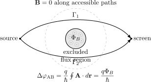
Two paths enclose an inaccessible flux region. The field can vanish along both paths while the closed-loop phase $\Delta\varphi_{\mathrm{AB}}=(q/\hbar)\oint\mathbf A\cdot d\mathbf r$ remains measurable through interference.

The effect is not a claim that a hidden Lorentz force acts along the exterior paths. In the ideal magnetic setup, the local force law sees $\mathbf E=\mathbf 0$ and $\mathbf B=\mathbf 0$ where the particle travels. The interference pattern sees the relative phase of amplitudes that wind differently around an excluded region.

Phase Shift

For a particle of charge $q$ minimally coupled to a vector potential, the Hamiltonian contains

$$\hat{\mathbf p} \longmapsto \hat{\mathbf p}-q\mathbf A.$$

Along a path $\Gamma$, the magnetic contribution to the quantum phase is

$$\varphi_\Gamma = \frac{q}{\hbar} \int_\Gamma \mathbf A\cdot d\mathbf r.$$

For two paths $\Gamma_1$ and $\Gamma_2$ with common endpoints, the observable phase difference is the closed-loop integral over $C=\Gamma_1-\Gamma_2$:

$$\begin{aligned} \Delta\varphi_{\mathrm{AB}} &= \frac{q}{\hbar} \left( \int_{\Gamma_1}\mathbf A\cdot d\mathbf r - \int_{\Gamma_2}\mathbf A\cdot d\mathbf r \right)\\ &= \frac{q}{\hbar} \oint_C \mathbf A\cdot d\mathbf r. \end{aligned}$$

If the loop encloses magnetic flux $\Phi_B$ with the chosen orientation, then

$$\oint_C \mathbf A\cdot d\mathbf r = \Phi_B,$$

so

$$\Delta\varphi_{\mathrm{AB}} = \frac{q\Phi_B}{\hbar} \quad \operatorname{mod} 2\pi.$$

The interference pattern is periodic under

$$\Phi_B \mapsto \Phi_B+\Phi_0, \qquad \Phi_0 = \frac{h}{\lvert q\rvert}.$$

For electrons, $q=-e$, so the sign of the phase depends on the loop orientation and charge convention. The physical fringe shift is the phase modulo $2\pi$.

Gauge Invariance

A gauge transformation changes the vector potential by

$$\mathbf A \mapsto \mathbf A+\nabla\chi,$$

and the wavefunction by a compensating local phase. With the convention $p\mapsto p-qA$,

$$\psi \mapsto \exp \left( \frac{iq\chi}{\hbar} \right) \psi.$$

For an open path, the line integral changes by an endpoint term:

$$\int_\Gamma \left( \mathbf A+\nabla\chi \right)\cdot d\mathbf r = \int_\Gamma \mathbf A\cdot d\mathbf r + \chi(b)-\chi(a).$$

That is why a single open-path phase is not separately gauge invariant. In an interference experiment the endpoint phase changes are also carried by the transformed wavefunctions, so the physical relative phase is unchanged.

For a closed loop and a single-valued gauge function,

$$\oint_C \nabla\chi\cdot d\mathbf r = 0.$$

Thus the phase factor

$$W(C) = \exp \left( \frac{iq}{\hbar} \oint_C \mathbf A\cdot d\mathbf r \right)$$

is gauge invariant. This loop phase is the abelian Wilson loop of the electromagnetic connection in nonrelativistic quantum mechanics.

Topological Character

The essential geometry is not that $\mathbf B$ is nonzero on the particle path. It is that the accessible configuration space has a hole. In the idealized planar setup, the particle moves in the punctured plane

$$M = \mathbb R^2\setminus\{0\},$$

or, more realistically, in the complement of a finite-radius flux tube. Loops in $M$ are labeled by an integer winding number around the excluded region.

A convenient exterior vector potential for a thin flux tube is

$$\mathbf A = \frac{\Phi_B}{2\pi r} \hat{\boldsymbol\theta}.$$

For $r>0$,

$$\nabla\times\mathbf A = \mathbf 0,$$

but a counterclockwise circle of radius $r$ has

$$\begin{aligned} \oint \mathbf A\cdot d\mathbf r &= \int_0^{2\pi} \frac{\Phi_B}{2\pi r} \left( r\,d\theta \right)\\ &= \Phi_B. \end{aligned}$$

For a loop with winding number $w$,

$$\oint_C \mathbf A\cdot d\mathbf r = w\Phi_B, \qquad \Delta\varphi_{\mathrm{AB}} = \frac{qw\Phi_B}{\hbar}.$$

This is the simplest quantum-mechanical example of a flat connection with nontrivial holonomy. Locally, the connection can look pure gauge. Globally, a loop that winds around the removed region cannot be shrunk to a point without leaving the accessible space.

The phrase “topological” needs some care. The winding number is topological, and the phase is insensitive to smooth deformations of the paths that preserve the winding and avoid the flux. The phase is not quantized by topology alone; it varies continuously with $\Phi_B$ and becomes physically periodic only modulo the flux quantum.

Stokes Theorem and the Missing Surface

A common paradox is to combine $\nabla\times\mathbf A=0$ outside the solenoid with Stokes theorem and conclude that the loop integral must vanish. The missing assumption is the existence of a smooth surface in the accessible region whose boundary is the loop and on which the same smooth vector potential is defined.

For a loop that winds around the excluded flux tube, every spanning disk crosses the removed region. If one allows a surface that cuts through the solenoid, then the magnetic field through the excluded core contributes:

$$\oint_C \mathbf A\cdot d\mathbf r = \int_\Sigma \mathbf B\cdot d\mathbf S = \Phi_B.$$

If one restricts to the accessible region, no such disk exists for a winding loop. That is the topology. Stokes theorem is not failing; its hypotheses are being violated by the puncture or by the need for multiple patches.

Relation to Berry Phase

The Aharonov–Bohm phase and Berry phase are both closed-loop phases, but their connections live over different spaces.

In the Aharonov–Bohm effect, the connection is the electromagnetic vector potential over the particle’s configuration space. The loop is a real-space loop around excluded flux:

$$\gamma_{\mathrm{AB}}[C] = \frac{q}{\hbar} \oint_C \mathbf A\cdot d\mathbf r.$$

In Berry phase, the connection is built from parameter-dependent eigenvectors:

$$\mathbf A_n(R) = i\langle n(R)|\nabla_R n(R)\rangle, \qquad \gamma_n[C] = \oint_C \mathbf A_n(R)\cdot dR.$$

The shared word is holonomy: a phase remains after transporting around a closed loop. The difference is physical origin. Aharonov–Bohm phase is electromagnetic gauge holonomy in configuration space; Berry phase is eigenstate-bundle holonomy in parameter space under adiabatic evolution.

There is also a useful contrast in curvature. In many Berry examples, a nonzero local Berry curvature contributes to the phase through a surface flux. In the ideal magnetic Aharonov–Bohm exterior, the local magnetic field strength vanishes on the accessible region, but the space is not simply connected. This makes the Aharonov–Bohm effect a clean reminder that zero local curvature does not always imply trivial global holonomy.

Experimental Significance

The effect was proposed by Aharonov and Bohm in 1959 and observed in electron interference experiments soon after. Later experiments with improved shielding addressed the worry that stray magnetic fields or forces were responsible for the fringe shift.

The modern lesson is not that gauge choices themselves are observable. It is that electromagnetic gauge potentials encode global phase information whose gauge-invariant content can appear in interference. This lesson reappears in mesoscopic rings, persistent currents, superconducting flux quantization, quantum Hall systems, and topological phases of matter.

The electric Aharonov–Bohm effect is a related effect involving scalar potentials and time-dependent phases. This page focuses on the magnetic case because it most directly displays holonomy around an excluded region.

Common Mistakes

• Saying $\mathbf A$ itself is directly observable. The gauge-invariant object is the closed-loop phase factor.
• Treating $\mathbf B=0$ along the paths as implying zero phase. The loop can enclose flux outside the accessible region.
• Applying Stokes theorem on a spanning surface that crosses an excluded region without accounting for the flux there.
• Forgetting the charge sign and loop orientation when comparing formulas.
• Calling the phase purely topological. The winding class is topological, but the phase also depends continuously on $\Phi_B$ modulo $\Phi_0$.
• Confusing Aharonov–Bohm holonomy in real space with Berry holonomy in parameter space.

Cross-Links

• Aharonov–Bohm Effect: First Encounter gives the wave-mechanics derivation and ring-spectrum first encounter.
• Minimal Coupling in Wave Mechanics explains the $p-qA$ replacement.
• Gauge Transformations: First Encounter gives the local phase transformation law.
• Magnetic Translations explains the flux phase in the translation algebra of uniform magnetic fields.
• Dirac Monopole Preview uses the same loop-phase logic to explain monopole quantization and patching.
• Particle on a Ring gives the exactly solvable flux-threaded ring model.
• Aharonov–Bohm Rings develops the open-conductor experiment: magnetoconductance harmonics, field-to-area calibration, phase rigidity, and dephasing controls.
• Periodic Boundary Conditions explains the twisted-boundary-condition viewpoint.
• Holonomy gives the general loop-transport language.
• Homotopy and Winding explains why winding classes matter.
• U(1) Bundles and Quantum Phase gives the phase-bundle perspective.
• Berry Phase compares geometric phases from adiabatic parameter loops.
• Berry Phase in the Aharonov–Bohm Effect explains the shared holonomy language and the important differences.
• Berry Phase Problems includes solved Aharonov–Bohm holonomy and winding checks.
• From Phase Symmetry to Gauge Theory connects this loop phase to the broader gauge-theory bridge.
• From Berry Phase to Topological Terms explains how loop phases become action terms and winding-sector weights.

References

• Y. Aharonov and D. Bohm, “Significance of electromagnetic potentials in the quantum theory,” Physical Review 115, 485-491, 1959.
• R. G. Chambers, “Shift of an electron interference pattern by enclosed magnetic flux,” Physical Review Letters 5, 3-5, 1960.
• A. Tonomura et al., “Evidence for Aharonov–Bohm effect with magnetic field completely shielded from electron wave,” Physical Review Letters 56, 792-795, 1986.
• M. Peshkin and A. Tonomura, The Aharonov–Bohm Effect, Springer, 1989.
• M. V. Berry, “Quantal phase factors accompanying adiabatic changes,” Proceedings of the Royal Society A 392, 45-57, 1984.
• J. J. Sakurai and J. Napolitano, Modern Quantum Mechanics, 3rd ed., Cambridge University Press, 2020.

Exercises

1. Compute the loop integral for the thin-flux-tube potential.

Let

$$\mathbf A = \frac{\Phi_B}{2\pi r} \hat{\boldsymbol\theta}$$

for $r>0$. Show that a counterclockwise circle centered on the flux tube has Aharonov–Bohm phase $q\Phi_B/\hbar$.

Solution

On a circle of radius $r$, the displacement is

$$d\mathbf r = r\,d\theta\,\hat{\boldsymbol\theta}.$$

Therefore

$$\begin{aligned} \oint \mathbf A\cdot d\mathbf r &= \int_0^{2\pi} \frac{\Phi_B}{2\pi r} r\,d\theta\\ &= \Phi_B. \end{aligned}$$

The phase is

$$\Delta\varphi_{\mathrm{AB}} = \frac{q}{\hbar} \oint \mathbf A\cdot d\mathbf r = \frac{q\Phi_B}{\hbar}.$$

2. Show gauge invariance of the closed-loop phase.

Suppose $\mathbf A\mapsto\mathbf A+\nabla\chi$ with a single-valued $\chi$ on the loop. Show that $W(C)$ is unchanged.

Solution

The exponent changes by

$$\frac{iq}{\hbar} \oint_C \nabla\chi\cdot d\mathbf r.$$

Along the closed loop, this integral is

$$\chi(\text{endpoint})-\chi(\text{startpoint}) = 0$$

for a single-valued $\chi$. Hence

$$W(C) = \exp \left( \frac{iq}{\hbar} \oint_C \mathbf A\cdot d\mathbf r \right)$$

is unchanged.

3. Include winding number.

A loop winds $w$ times around the excluded flux region. What is the phase, and what flux change leaves the interference pattern invariant?

Solution

The loop integral is multiplied by the winding number:

$$\oint_C \mathbf A\cdot d\mathbf r = w\Phi_B.$$

Thus

$$\Delta\varphi_{\mathrm{AB}} = \frac{qw\Phi_B}{\hbar}.$$

The interference pattern is unchanged when the phase changes by $2\pi k$ with $k\in\mathbb Z$. For one winding, the smallest positive flux period in magnitude is

$$\Phi_0 = \frac{h}{\lvert q\rvert}.$$

For fixed winding $w\ne0$, changing the flux by $\Phi_0/\lvert w\rvert$ changes this loop phase by $2\pi$ in magnitude, although the fundamental flux periodicity of a system containing all allowed winding sectors remains $\Phi_0$.

4. Compare Aharonov–Bohm and Berry phases.

Give one similarity and one difference between the two phases.

Solution

A similarity is that both are holonomies: they are phases associated with closed-loop transport and are physically meaningful modulo $2\pi$.

A difference is the base space and connection. The Aharonov–Bohm phase comes from the electromagnetic vector potential over real configuration space. Berry phase comes from a connection built from parameter-dependent eigenvectors over parameter space, usually under an adiabatic assumption.