Aharonov–Bohm Rings

An Aharonov–Bohm ring is an open mesoscopic conductor in which electrons can travel between reservoirs through two or more paths that enclose magnetic flux. The terminal conductance oscillates because the relative phase of those paths changes by $2\pi$ when the enclosed flux changes by the normal-electron flux quantum $h/e$.

The ideal Aharonov–Bohm thought experiment isolates flux from the accessible paths. A laboratory ring is usually placed in a nearly uniform magnetic field, so the field also penetrates the arms and leads. Orbital deflection, Zeeman splitting, weak localization, universal conductance fluctuations, contact motion, and density changes can accompany the flux phase. A periodic trace is therefore a mesoscopic inference problem, not a literal image of two force-free trajectories.

This page owns ring magnetotransport: two-arm interference, conductance harmonics, field-to-area calibration, $h/e$ and $h/2e$ mechanisms, two-terminal phase rigidity, ring-specific coherence extraction, and Fourier-analysis controls. Aharonov–Bohm Effect owns the gauge-holonomy and topology derivation. Aharonov–Bohm Effect: First Encounter owns the wave-mechanics and closed-ring spectrum. Quantum Coherence in Conductors owns the generic dephasing kernel and comparison among coherence extractors.

Ring Geometry and Phase

Consider source and drain reservoirs connected by upper and lower arms. Let $\Phi$ be the magnetic flux through an oriented effective ring area. For charge $q$, the electromagnetic contribution to the relative phase is

$$\Delta\varphi_{\mathrm{AB}} = \frac{q}{\hbar} \oint_C \mathbf A\cdot d\mathbf r = \frac{q\Phi}{\hbar}.$$

Define the positive normal-electron flux quantum

$$\Phi_0 \equiv \frac{h}{e} \approx 4.1357\times10^{-15}\,\mathrm{Wb}.$$

For an electron, $q=-e$, so orientation fixes the sign:

$$\Delta\varphi_{\mathrm{AB}} = -2\pi\frac{\Phi}{\Phi_0} \pmod{2\pi}.$$

The measured oscillation period is insensitive to that sign. The sign matters when combining magnetic phase with dynamical, spin, valley, or Berry phases under a declared orientation convention.

The total phase difference between two arms is

$$\Delta\varphi(E,B) = \Delta\varphi_{\mathrm{dyn}}(E,B) +\Delta\varphi_{\mathrm{AB}}(B) +\Delta\varphi_{\mathrm{int}}(E,B),$$

where the last term can include spin rotation, geometric phase, scattering phases, or a resonant element embedded in one arm. Gate voltage can change path length, wave number, mode occupation, and junction scattering at the same time.

An open ring is not a closed-ring spectrum

The exactly solvable particle-on-a-ring problem has discrete flux-shifted energies and equilibrium persistent current. A conductance ring is open to reservoirs. Its observable is a scattering probability, broadened by escape and averaged over occupied energies. Both systems are flux periodic, but persistent current and two-terminal conductance are different observables with different ensembles and dissipation ledgers.

Particle on a Ring is the canonical home for the closed spectrum. The open-ring calculation begins with transmission amplitudes.

From Path Amplitudes to Conductance

In the simplest single-mode picture, write the source-to-drain amplitude as

$$t = t_u e^{i\varphi_u} +t_\ell e^{i\varphi_\ell}.$$

Then

$$\begin{aligned} T ={}& \lvert t\rvert^2 \\ ={}& T_u+T_\ell +2\sqrt{T_uT_\ell} \cos\Delta\varphi, \end{aligned}$$

where $T_u=\lvert t_u\rvert^2$, $T_\ell=\lvert t_\ell\rvert^2$, and $\Delta\varphi=\varphi_u-\varphi_\ell$. At zero temperature, one resolved channel contributes

$$G = \frac{e^2}{h}T.$$

This two-path formula explains the oscillation, but real junctions permit reflection and repeated winding. The amplitude then contains paths labeled by arm sequence, transverse mode, spin, and winding number. A useful schematic expansion is

$$t_{\mathrm{tot}} = \sum_p a_p \exp \left[ i\varphi_p^{(0)} +i2\pi w_p\frac{\Phi}{\Phi_0} \right],$$

where $w_p\in\mathbb Z$ is the oriented winding number. Conductance contains cross terms between every pair of paths that arrive in the same outgoing channel.

Visibility is not a pure coherence meter

For a nearly sinusoidal trace, an experimental visibility is often defined as

$$\mathcal V \equiv \frac{G_{\max}-G_{\min}} {G_{\max}+G_{\min}}.$$

In the ideal two-path model,

$$\mathcal V_{\mathrm{ideal}} = \frac{ 2\sqrt{T_uT_\ell} }{ T_u+T_\ell }.$$

Perfect coherence therefore does not guarantee unit visibility: strongly unequal arm amplitudes reduce contrast. Mode averaging, contact reflection, path-length mismatch, finite temperature, detector bandwidth, and background conductance also reduce it. Extracting a phase-coherence length from visibility requires a transport model and control of those non-dephasing factors.

Flux Period and Effective Area

One additional flux quantum changes the single-winding phase by $2\pi$:

$$\Delta\Phi = \Phi_0.$$

If a perpendicular field threads an effective area $A_{\mathrm{eff}}$, then

$$\Phi \approx BA_{\mathrm{eff}}, \qquad \Delta B_{h/e} = \frac{\Phi_0}{A_{\mathrm{eff}}}.$$

A measured period therefore gives

$$A_{\mathrm{eff}} = \frac{\Phi_0}{\Delta B_{h/e}}, \qquad r_{\mathrm{eff}} = \sqrt{ \frac{A_{\mathrm{eff}}}{\pi} }$$

for a circular-area comparison. The effective area need not equal the area inside a lithographic centerline. Finite arm width provides a distribution of enclosed areas, while depletion, edge states, magnetic focusing, flux focusing, and density-dependent path motion shift the conducting trajectories.

For an annulus with inner and outer radii $r_i$ and $r_o$, plausible orbital areas span

$$\pi r_i^2 \lesssim A \lesssim \pi r_o^2.$$

A broad or split Fourier peak can therefore be geometric rather than evidence for two independent particles or two topological sectors.

Byers–Yang periodicity

For particles of charge magnitude $e$ in a multiply connected normal system, gauge invariance implies periodicity under insertion of $h/e$ flux, including in the presence of interactions when the many-body state and boundary conditions are treated consistently. This fundamental periodicity does not require every measured trace to be a single sinusoid.

The conductance may contain harmonics:

$$\delta G(B) = \sum_{n=1}^{\infty} A_n \cos \left( 2\pi n \frac{BA_{\mathrm{eff}}}{\Phi_0} +\phi_n \right).$$

The $n$th harmonic has field period

$$\Delta B_n = \frac{\Phi_0}{nA_{\mathrm{eff}}}.$$

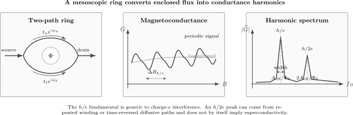
Upper and lower arm amplitudes acquire a relative phase $2\pi\Phi/\Phi_0$ and recombine at the drain. A field sweep produces oscillatory conductance on top of a generally nonperiodic background. Fourier analysis can reveal an $h/e$ peak and higher winding or time-reversed $h/2e$ structure, but peak width also records the finite field window and distribution of effective ring areas.

h/e and h/2e Harmonics

The same field period can arise from different path families, so harmonic labels are not mechanism labels by themselves.

Sample-specific h/e oscillations

Interference between paths whose winding numbers differ by one gives the $h/e$ period. In a disordered ring, its phase depends on the particular impurity configuration and Fermi energy. Averaging over many independent disorder realizations, rings, or sufficiently broad gate ranges can suppress the signed $h/e$ contribution even when each individual ring shows it clearly.

Repeated winding

A coherent path that circles twice before leaving can interfere with a path whose winding differs by two, producing an $h/2e$ harmonic. Higher harmonics similarly probe longer dwell paths and are usually more sensitive to dephasing and escape.

Altshuler–Aronov–Spivak oscillations

In a diffusive ring or cylinder, a path and its time reverse accumulate the same random dynamical phase but opposite magnetic phase. Their interference contribution depends on

$$2\Delta\varphi_{\mathrm{AB}} = 4\pi\frac{\Phi}{\Phi_0},$$

and therefore has period $h/2e$. Because static-disorder phases cancel for this time-reversed pair, the ensemble-averaged contribution can survive when the sample-specific $h/e$ term averages toward zero.

This is the ring analogue of the Cooperon channel in weak localization. It is distinct from superconducting $h/2e$ flux periodicity, where the condensate charge is $2e$. Observing an $h/2e$ peak in a normal ring does not by itself imply pairing.

Observed component	Representative origin	Disorder averaging
$h/e$	paths whose winding differs by one	phase is generally sample specific
$h/2e$	double winding in one sample	can remain sample specific
$h/2e$	time-reversed diffusive loops	survives ensemble averaging more robustly
$h/2e$ in a superconductor	charge-$2e$ condensate response	different physical origin

Phase Rigidity and Terminal Geometry

Linear-response reciprocity gives

$$G_{ij}(B) = G_{ji}(-B)$$

when microscopic reversibility applies and magnetic order or other time-reversal-breaking controls are reversed consistently. In a two-terminal conductor this reduces to

$$G(B) = G(-B).$$

Suppose an isolated first harmonic is written

$$\delta G_1(B) = A_1 \cos \left( 2\pi\frac{BA_{\mathrm{eff}}}{\Phi_0} +\phi_1 \right).$$

Evenness in $B$ requires

$$\phi_1 = 0 \quad\text{or}\quad \pi \pmod{2\pi}.$$

This phase rigidity means that the apparent two-terminal oscillation phase cannot generally slide continuously under a gate sweep while remaining a single linear-response harmonic. Its amplitude can pass through zero and reappear with a $\pi$ jump.

The restriction changes in a multi-terminal interferometer because reciprocity relates different lead permutations rather than forcing one trace to be even. Nonlinear conductance can also contain field-antisymmetric terms. Terminal geometry and bias regime must therefore be reported before interpreting an oscillation phase as the transmission phase of a quantum dot or other embedded object.

Symmetrizing a noisy trace by hand can conceal a real nonlinear or multi-terminal asymmetry. Reciprocity is a physical test to perform on the raw linear-response data, not merely a plotting instruction.

Ballistic and Diffusive Rings

In a ballistic or quasiballistic ring, a small number of arm modes and junction scattering amplitudes may dominate. Gate-defined quantum point contacts can tune injection and beam-splitter balance. Semiclassical path lengths and mode conversion then organize the interference.

In a diffusive ring,

$$\ell_e \ll P,$$

where $P$ is the circumference. Many elastically scattered paths contribute. Static disorder does not automatically destroy coherence; it fixes a reproducible interference fingerprint. The useful distinction is

$$\ell_e \quad\text{versus}\quad L_\phi:$$

$\ell_e$ controls momentum randomization, while $L_\phi$ controls phase memory. A ring can be diffusive and phase coherent when

$$\ell_e \ll P \lesssim L_\phi.$$

Contacts introduce an escape time and can truncate long winding paths before intrinsic dephasing does. Closing the contacts raises dwell time and harmonic content but can also create resonances or an unintended quantum dot. A complete ring model includes arm disorder, junction scattering, reservoir coupling, and mode number.

Dephasing and Thermal Averaging

For a one-winding path length $P$, a common phenomenological harmonic envelope is

$$A_n(T) \sim A_n^{(0)} R_{T,n} R_{\mathrm{esc},n} \exp \left( -\frac{nP}{L_\phi(T)} \right).$$

$R_{T,n}$ describes thermal and energy averaging, while $R_{\mathrm{esc},n}$ describes loss through contacts. The exponential form is a useful diagnostic, not a universal theorem. Ballistic and diffusive rings weight path times differently; spin, intervalley structure, ring arrays, canonical versus grand-canonical conditions, and nonexponential phase noise can change the prefactor and exponent.

The thermal length is often estimated as

$$L_T^{\mathrm{diff}} = \sqrt{ \frac{\hbar D}{k_{\mathrm B}T} }$$

in diffusion, or parametrically

$$L_T^{\mathrm{bal}} \sim \frac{\hbar v_F}{k_{\mathrm B}T}$$

for ballistic energy averaging. Numerical factors depend on the observable and geometry.

Thermal averaging is not dephasing

At finite temperature, linear conductance averages the energy-dependent transmission:

$$G(T) = \frac{e^2}{h} \int dE\, \left( -\frac{\partial f}{\partial E} \right) T(E).$$

If the interference phase changes across the Fermi window, contributions at different energies cancel in the measured average even though each electron remains coherent. True dephasing instead reduces phase correlations through inelastic scattering, fluctuating environments, or entanglement with unobserved degrees of freedom.

Changing temperature affects both. A credible extraction of $L_\phi(T)$ either models $R_T$ independently, compares harmonics and ring sizes, or uses another coherence observable. Fitting all amplitude loss to $\exp(-P/L_\phi)$ overestimates intrinsic dephasing.

Why higher harmonics help

Under the simple common-prefactor model,

$$\frac{A_{n+1}}{A_n} \propto \exp \left( -\frac{P}{L_\phi} \right).$$

Higher windings therefore amplify sensitivity to phase memory. But their junction amplitudes, thermal factors, and effective areas need not match. Harmonic ratios become quantitative only after those assumptions are tested.

Measurement and Fourier Workflow

Establish the regime

Report ring radii and arm width, carrier density, $\ell_e$, $L_\phi$, temperature, excitation bias, lead number, and contact transparency. State whether the transport is ballistic, quasiballistic, diffusive, or resonant.

Verify linear response and reciprocity

Reduce the excitation until the trace is bias independent within uncertainty. Compare $G(B)$ and $G(-B)$ before background subtraction. A two-terminal linear trace should be even apart from drift and noise.

Separate periodic signal from background

Classical magnetoresistance, weak localization, and conductance fluctuations can be larger than the ring oscillation. Detrending must preserve periods near the expected $\Delta B$. Report the polynomial, smoothing scale, or high-pass filter and demonstrate robustness against reasonable alternatives.

Use a controlled Fourier transform

For uniformly sampled field points $B_j$, transform a declared window of $\delta G(B_j)$. The finite field span $\mathcal B$ limits frequency resolution to order

$$\delta f_B \sim \frac{1}{\mathcal B}.$$

Window functions trade spectral leakage for peak width. Zero padding interpolates the displayed spectrum but does not improve physical resolution. Quote the field range, sampling interval, window, and frequency-to-area conversion.

Test effective area

Compare

$$A_{\mathrm{FFT}} = f_B\Phi_0$$

with the geometric annulus. Track the peak versus gate voltage. Smooth motion can reflect a changing electronic path; abrupt jumps can reflect mode switching or charge rearrangement.

Check reproducibility without averaging away the physics

Repeat sweeps in both directions and at several rates. Warm cycling may rearrange disorder and change the $h/e$ fingerprint while preserving its characteristic period. An array average can enhance the disorder-robust $h/2e$ component and suppress sample-specific $h/e$ oscillations.

Observation	Strong interpretation	Essential control
peak at $A/\Phi_0$	one-winding flux interference	match area and track gate dependence
peak at $2A/\Phi_0$	$h/2e$ harmonic	distinguish double winding, AAS, and pairing
amplitude falls with $T$	reduced coherent contrast	separate thermal averaging from dephasing
apparent continuous phase shift	path or scatterer phase evolution	check terminal geometry and phase rigidity
split Fourier peak	several effective areas or beating	vary field window, gate voltage, and detrending
oscillations survive large field	robust phase-coherent paths	audit field penetration, Zeeman, and edge reconstruction

Berry Phase and Topology

Aharonov–Bohm and Berry phases share the mathematics of a $U(1)$ holonomy, but their base spaces and physical assumptions differ.

Feature	Aharonov–Bohm phase	Berry phase
connection	electromagnetic $\mathbf A(\mathbf r)$	eigenstate connection in parameter or momentum space
loop	real-space path around flux	adiabatic path of an eigenspace
basic assumption	coherent path interference	adiabatic following
curvature	magnetic field, possibly excluded from paths	Berry curvature in the chosen bundle

Berry Phase in the Aharonov–Bohm Effect owns the detailed comparison.

Spin–orbit coupling can rotate spin around a ring and add an Aharonov–Casher or spin geometric phase. In a topological-insulator nanowire, a surface-state Berry phase can shift which flux values close the finite-size gap. These are additional structures layered on the ordinary electromagnetic phase.

An $h/e$ conductance oscillation alone is not evidence of topological matter: conventional normal-metal and semiconductor rings show the same fundamental period. A topological claim needs the predicted phase or parity pattern, surface or edge-state identification, disorder and density dependence, and consistency with the material’s band topology. Even then, Zeeman energy, bulk conduction, finite thickness, and multiple areas must be modeled.

The word topological also has two meanings to keep separate. The ideal Aharonov–Bohm geometry is multiply connected, so winding classes are topological. The phase itself varies continuously with flux and does not by itself define a topological phase of matter.

Common Mistakes

Treating uniform-field rings as perfectly field free

The field threads the arms and leads, so orbital and Zeeman effects can accompany the flux phase.

Using the lithographic hole as the exact area

Finite-width trajectories, depletion, edge motion, and focusing define $A_{\mathrm{eff}}$.

Calling every h/2e peak superconducting

Double winding and Altshuler–Aronov–Spivak interference produce $h/2e$ structure in normal conductors.

Equating reduced visibility with dephasing

Arm imbalance, thermal averaging, mode averaging, escape, and drift also reduce contrast.

Reading a continuous phase from a closed two-terminal trace

Linear-response phase rigidity constrains a single harmonic to phase $0$ or $\pi$.

Letting zero padding masquerade as resolution

The physical Fourier resolution is set by the measured field span, not by the number of interpolated frequency points.

Averaging away sample-specific h/e oscillations

Disorder or gate averaging can suppress the first harmonic while preserving an $h/2e$ ensemble contribution.

Calling an h/e period a topological-material signature

The period is generic electromagnetic interference; topology requires additional phase, state, and material evidence.

Exercises

1. Derive the ideal visibility

Starting from two arm probabilities $T_u$ and $T_\ell$, derive $\mathcal V_{\mathrm{ideal}}$. Evaluate it for $T_u=0.64$ and $T_\ell=0.16$.

Solution

The extrema of

$$T = T_u+T_\ell +2\sqrt{T_uT_\ell}\cos\Delta\varphi$$

are

$$T_{\max,\min} = T_u+T_\ell \pm 2\sqrt{T_uT_\ell}.$$

Therefore

$$\mathcal V_{\mathrm{ideal}} = \frac{T_{\max}-T_{\min}} {T_{\max}+T_{\min}} = \frac{2\sqrt{T_uT_\ell}} {T_u+T_\ell}.$$

For the stated values,

$$\mathcal V_{\mathrm{ideal}} = \frac{2\sqrt{(0.64)(0.16)}}{0.80} = 0.80.$$

The paths can be fully coherent even though their unequal amplitudes prevent unit visibility.

2. Infer an effective radius

An $h/e$ oscillation has period $\Delta B=25\,\mathrm{mT}$. Find $A_{\mathrm{eff}}$ and the corresponding circular radius.

Solution

Using $\Phi_0=4.1357\times10^{-15}\,\mathrm{Wb}$,

$$A_{\mathrm{eff}} = \frac{\Phi_0}{\Delta B} \approx \frac{4.1357\times10^{-15}} {2.5\times10^{-2}} \approx 1.65\times10^{-13}\,\mathrm{m^2}.$$

Then

$$r_{\mathrm{eff}} = \sqrt{\frac{A_{\mathrm{eff}}}{\pi}} \approx 2.30\times10^{-7}\,\mathrm m = 230\,\mathrm{nm}.$$

This radius should be compared with the full conducting annulus, not only the drawn gate centerline.

3. Locate two harmonics

A ring has $A_{\mathrm{eff}}=0.50\,\mu\mathrm m^2$. Find the $h/e$ and $h/2e$ field periods.

Solution

Since $0.50\,\mu\mathrm m^2=5.0\times10^{-13}\,\mathrm{m^2}$,

$$\Delta B_{h/e} = \frac{\Phi_0}{A_{\mathrm{eff}}} \approx 8.27\,\mathrm{mT}.$$

The second harmonic has half that period:

$$\Delta B_{h/2e} = \frac{\Phi_0}{2A_{\mathrm{eff}}} \approx 4.14\,\mathrm{mT}.$$

The period identifies the harmonic, not whether its microscopic origin is double winding or an AAS path pair.

4. Prove phase rigidity for one harmonic

Show that $G(B)=G(-B)$ forces $\phi=0$ or $\pi$ for

$$\delta G = A\cos \left( 2\pi BA_{\mathrm{eff}}/\Phi_0+\phi \right)$$

when $A\neq0$.

Solution

Let $\theta=2\pi BA_{\mathrm{eff}}/\Phi_0$. Evenness requires

$$\cos(\theta+\phi) = \cos(-\theta+\phi)$$

for all $\theta$. Their difference is

$$-2\sin\phi\sin\theta.$$

It vanishes for every $\theta$ only if $\sin\phi=0$, hence

$$\phi = 0 \quad\text{or}\quad \pi \pmod{2\pi}.$$

If $A$ passes through zero during a gate sweep, the fitted phase can jump by $\pi$ without violating reciprocity.

5. Why can h/2e survive averaging?

Explain why an ensemble of disordered rings can lose its average $h/e$ signal while retaining an $h/2e$ component.

Solution

The $h/e$ phase contains sample-specific dynamical phases fixed by each disorder realization, so its signed contribution averages toward zero across many statistically independent rings or configurations. For a path paired with its time reverse, the static-disorder phase is the same and cancels in the relative phase, while the magnetic phase doubles. This disorder-robust pair produces an Altshuler–Aronov–Spivak contribution with period $h/2e$.

6. Estimate a coherence length from harmonics

Assume

$$A_n = C \exp \left( -\frac{nP}{L_\phi} \right)$$

with the same prefactor $C$ for two harmonics. A ring has $P=1.5\,\mu\mathrm m$ and $A_2/A_1=0.25$. Find $L_\phi$.

Solution

The ratio is

$$\frac{A_2}{A_1} = \exp \left( -\frac{P}{L_\phi} \right) = 0.25.$$

Thus

$$L_\phi = \frac{P}{\ln4} \approx \frac{1.5\,\mu\mathrm m}{1.386} \approx 1.08\,\mu\mathrm m.$$

This estimate fails if the two harmonics have different junction, thermal, area, or escape prefactors.

7. Separate thermal averaging from dephasing

The $h/e$ amplitude falls rapidly with temperature. Give four measurements that help decide whether $L_\phi$ is shrinking or energy averaging is dominant.

Solution

Useful controls include measuring rings with different circumference, comparing several harmonic ratios, extracting an independent $L_\phi$ from weak localization or conductance correlations, measuring electron temperature, varying arm-length imbalance, and acquiring energy or gate-correlation data to determine how rapidly the interference phase changes across the Fermi window. A model should convolve the energy-dependent transmission with $-\partial f/\partial E$ before assigning the remaining decay to dephasing.

8. Audit a topological-ring claim

A nanowire shows an $h/e$ magnetoconductance peak. Why is that insufficient to establish topological surface transport, and what additional evidence is needed?

Solution

Ordinary metallic and semiconductor rings also show $h/e$ interference. A stronger case requires the predicted flux-dependent phase or parity pattern, gate evolution tied to surface-state occupancy, independent evidence for the relevant surface or edge bands, robustness and disorder trends consistent with the proposed model, and exclusion of bulk channels, Zeeman-driven changes, multiple effective areas, and ordinary universal conductance fluctuations. The period is necessary for the proposed interference picture but not diagnostic of band topology by itself.

Connections

• Aharonov–Bohm Effect owns electromagnetic gauge holonomy, winding, Stokes-theorem subtleties, and the precise topological statement.
• Aharonov–Bohm Effect: First Encounter derives the phase in wave mechanics and introduces the flux-shifted closed ring.
• Particle on a Ring develops the exact closed-system spectrum, twisted boundary conditions, and persistent-current interpretation.
• Quantum Coherence in Conductors owns dephasing mechanisms, coherence lengths, thermal averaging, and comparison among weak localization, fluctuations, and ring harmonics.
• Weak Localization treats the broad ensemble of time-reversed diffusive loops and its nonperiodic low-field cusp.
• Universal Conductance Fluctuations owns the reproducible aperiodic background, its covariance, symmetry crossover, and disorder-averaging controls.
• What Is Mesoscopic Physics? supplies the wavelength, mean-free-path, thermal, coherence, dwell, and geometry hierarchy.
• Quantum Point Contacts develops tunable beam splitters, transmission, partition noise, and detector backaction.
• Conductance Quantization owns the Landauer channel formula, terminal conventions, and contact resistance.
• Berry Phase in the Aharonov–Bohm Effect compares electromagnetic and eigenstate holonomies.
• Dephasing Versus Dissipation separates loss of phase information from energy relaxation in open-system language.
• Topological Insulators owns bulk $\mathbb Z_2$ topology and anomalous surface states.

Further Reading

• S. Washburn and R. A. Webb, “Aharonov–Bohm Effect in Normal Metal: Quantum Coherence and Transport,” Advances in Physics 35, 375–422 (1986), doi:10.1080/00018738600101921.
• A. G. Aronov and Yu. V. Sharvin, “Magnetic Flux Effects in Disordered Conductors,” Reviews of Modern Physics 59, 755–779 (1987), doi:10.1103/RevModPhys.59.755.
• Y. Imry, Introduction to Mesoscopic Physics, 2nd ed., Oxford University Press, 2002.
• S. Datta, Electronic Transport in Mesoscopic Systems, Cambridge University Press, 1995.

References

1. Y. Aharonov and D. Bohm, “Significance of Electromagnetic Potentials in the Quantum Theory,” Physical Review 115, 485–491 (1959), doi:10.1103/PhysRev.115.485.
2. N. Byers and C. N. Yang, “Theoretical Considerations Concerning Quantized Magnetic Flux in Superconducting Cylinders,” Physical Review Letters 7, 46–49 (1961), doi:10.1103/PhysRevLett.7.46.
3. B. L. Altshuler, A. G. Aronov, and B. Z. Spivak, “The Aharonov–Bohm Effect in Disordered Conductors,” JETP Letters 33, 94–97 (1981).
4. M. Büttiker, Y. Imry, R. Landauer, and S. Pinhas, “Generalized Many-Channel Conductance Formula with Application to Small Rings,” Physical Review B 31, 6207–6215 (1985), doi:10.1103/PhysRevB.31.6207.
5. R. A. Webb, S. Washburn, C. P. Umbach, and R. B. Laibowitz, “Observation of $h/e$ Aharonov–Bohm Oscillations in Normal-Metal Rings,” Physical Review Letters 54, 2696–2699 (1985), doi:10.1103/PhysRevLett.54.2696.
6. A. Yacoby, M. Heiblum, D. Mahalu, and H. Shtrikman, “Coherence and Phase Sensitive Measurements in a Quantum Dot,” Physical Review Letters 74, 4047–4050 (1995), doi:10.1103/PhysRevLett.74.4047.
7. A. Yacoby, R. Schuster, and M. Heiblum, “Phase Rigidity and $h/2e$ Oscillations in a Single-Ring Aharonov–Bohm Experiment,” Physical Review B 53, 9583–9586 (1996), doi:10.1103/PhysRevB.53.9583.
8. R. Schuster, E. Buks, M. Heiblum, D. Mahalu, V. Umansky, and H. Shtrikman, “Phase Measurement in a Quantum Dot via a Double-Slit Interference Experiment,” Nature 385, 417–420 (1997), doi:10.1038/385417a0.
9. A. E. Hansen, A. Kristensen, S. Pedersen, C. B. Sørensen, and P. E. Lindelof, “Mesoscopic Decoherence in Aharonov–Bohm Rings,” Physical Review B 64, 045327 (2001), doi:10.1103/PhysRevB.64.045327.
10. G. Seelig and M. Büttiker, “Charge-Fluctuation-Induced Dephasing in a Gated Mesoscopic Interferometer,” Physical Review B 64, 245313 (2001), doi:10.1103/PhysRevB.64.245313.
11. R. Leturcq et al., “Magnetic Field Symmetry and Phase Rigidity of the Nonlinear Conductance in a Ring,” Physical Review Letters 96, 126801 (2006), doi:10.1103/PhysRevLett.96.126801.
12. A. G. Aronov and Y. B. Lyanda-Geller, “Spin-Orbit Berry Phase in Conducting Rings,” Physical Review Letters 70, 343–346 (1993), doi:10.1103/PhysRevLett.70.343.
13. H. Peng et al., “Aharonov–Bohm Interference in Topological Insulator Nanoribbons,” Nature Materials 9, 225–229 (2010), doi:10.1038/nmat2609.
14. J. H. Bardarson, P. W. Brouwer, and J. E. Moore, “Aharonov–Bohm Oscillations in Disordered Topological Insulator Nanowires,” Physical Review Letters 105, 156803 (2010), doi:10.1103/PhysRevLett.105.156803.