Nanostructures for Quantum Technology

A nanostructure becomes a quantum technology only when a quantum effect can be turned into a repeatable, calibrated function inside a larger system. Confinement, interference, charge quantization, superconducting proximity, and topological band structure are enabling physics. They are not by themselves an architecture.

The engineering question is therefore not merely “is the device quantum?” It is:

Which state or observable carries the useful information, how is it initialized, controlled, coupled, measured, and reset, and how do all of those operations behave across devices and over time?

This page supplies a decision framework for answering that question. It owns the system ledger connecting materials and interfaces to an effective Hamiltonian, functional primitives, measured error channels, fabrication statistics, classical infrastructure, and task-level evidence. The microscopic derivations remain in their canonical homes: Quantum Dots owns confined addition spectra, Single-Electron Devices owns pumps and charge-transfer errors, Proximity and Andreev Physics owns hybrid-interface scattering, and Spin Qubits owns solid-state relaxation and dephasing.

The main lesson is deliberately sober: a record coherence time, a compact footprint, a high average fidelity, or a striking spectrum can each be important, but no one number establishes technological usefulness.

The Device-to-Architecture Ledger

Every credible proposal should be traceable through five layers.

Layer	Question	Minimum evidence
materials and interfaces	Which disorder, strain, traps, oxides, contacts, and reservoirs define the device?	process description, microscopy or spectroscopy where relevant, and statistics across nominally identical structures
effective Hamiltonian	Which low-energy states and couplings are retained, and where does that model fail?	measured spectrum, parameter extraction, leakage states, and uncertainty
functional primitives	How are states initialized, controlled, coupled, read, and reset?	pulse or bias protocol, bandwidth, timing, crosstalk, and repeated-operation data
calibrated error model	Which errors occur, with what correlations and drift?	SPAM, gate, idle, leakage, rare-event, and simultaneous-operation diagnostics
architecture and task	How are many primitives wired, calibrated, scheduled, and judged?	yield, thermal and classical budgets, connectivity, uptime, and a task-level metric

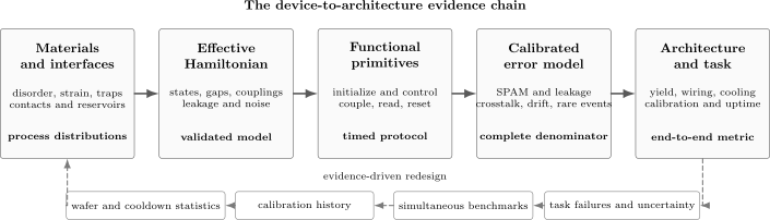
A quantum effect becomes a technology through a chain of measured interfaces. Forward arrows build the system; the lower feedback path represents redesign driven by wafer statistics, calibration histories, simultaneous benchmarks, and task failures. A claim that skips a layer is an invitation to find an unmeasured assumption.

The layers are coupled. Increasing a tunnel rate may accelerate reset but broaden a spectral line. A stronger electric dipole may improve control and resonator coupling while increasing charge-noise sensitivity. A larger superconducting gap may help thermal isolation while an imperfect interface adds subgap states. The correct design object is the whole ledger, not an isolated Hamiltonian parameter.

Begin with a Functional Specification

Information carrier and computational subspace

First state what is being stored or transported. Examples include:

• the spin projection of one electron;
• the singlet–triplet manifold of two spins;
• charge parity on an island;
• occupation of an Andreev level;
• the path or edge-channel index of a coherent carrier;
• one transferred electron per drive cycle; or
• a nonlocal parity in a candidate topological device.

Let $\mathcal H_{\mathrm{comp}}$ denote the intended subspace and $\mathcal H_{\mathrm{leak}}$ everything else that can be occupied. A useful device model has the form

$$H(t) = H_0 + \sum_a u_a(t)H_a + \sum_{\langle ab\rangle} H_{ab} + H_{\mathrm{noise}}(t).$$

Here $H_0$ fixes the idle spectrum, $u_a(t)H_a$ are controlled terms, $H_{ab}$ couples subsystems, and $H_{\mathrm{noise}}$ includes both environmental fluctuations and imperfect control. Writing this decomposition is easy. Establishing it experimentally requires spectroscopy, time-domain control, noise measurements, and checks for omitted levels.

The separation from the nearest unwanted level,

$$\Delta_{\mathrm{leak}} = \min_{n\in\mathcal H_{\mathrm{leak}}} \lvert E_n-E_{\mathrm{comp}}\rvert,$$

sets only one limit. Selection rules, matrix elements, pulse spectra, and interactions can make a nominally distant level important or a nearby level harmless.

Initialization and reset

Initialization prepares a known distribution; reset restores it quickly enough for reuse. These are different performance questions. Passive relaxation of a two-level system gives

$$p_e(t) = p_e^{\mathrm{eq}} + \left[ p_e(0)-p_e^{\mathrm{eq}} \right] e^{-t/T_1}.$$

Waiting several $T_1$ can be accurate but slow. Reservoir-assisted, measurement-based, or dissipative reset can be faster, but each introduces its own leakage, heating, and calibration dependencies. A reset specification should report the final state distribution, duration, conditional branches, and behavior under repetition.

For a level splitting $\hbar\omega_q$ in thermal equilibrium,

$$p_e^{\mathrm{eq}} = \frac{1} {1+\exp\!\left(\hbar\omega_q/k_BT\right)}.$$

This formula uses the effective temperature of the relevant degree of freedom, not merely the refrigerator thermometer. Microwave leakage, imperfect filtering, quasiparticles, reservoir bias, and slow relaxation can all produce a nonthermal population.

Control and coupling

A control must reach the desired operation before decoherence and drift dominate, while avoiding leakage and disturbing neighboring devices. The familiar ratio

$$Q_{\mathrm{op}} = \frac{T_2}{t_{\mathrm{op}}}$$

is a useful first diagnostic, not an operation count. It omits state-preparation and measurement errors, pulse imperfections, coherent accumulation, leakage, crosstalk, duty cycle, and the distinction among $T_2^*$, echo coherence, and driven coherence.

For a pulse of duration $\tau_p$, a rough spectral energy scale is $\hbar/\tau_p$. The schematic hierarchy

$$k_BT,\ \hbar\Gamma,\ \frac{\hbar}{\tau_p} \ll \Delta_{\mathrm{leak}}$$

is a helpful sufficient regime for thermal isolation, weak broadening, and spectrally selective control. It is not a universal design law. Shaped pulses can suppress selected transitions, and intentionally nonadiabatic protocols may cross small gaps in a controlled way.

Coupling is also a systems parameter. A nearest-neighbor interaction can be strong yet unusable if it cannot be turned off, calibrated independently, or scheduled without spectator errors. Report an on/off ratio, residual coupling, spatial range, tuning bandwidth, and sensitivity to the same controls used for single-device operations.

Readout

Readout converts a quantum state into a classical record. It should be characterized as a noisy measurement channel, not just by the separation of two histogram peaks. For binary state $s$ and reported outcome $m$, define the assignment matrix

$$M_{ms} = P(m\mid s) = \begin{pmatrix} P(0\mid0) & P(0\mid1)\\ P(1\mid0) & P(1\mid1) \end{pmatrix}.$$

Each column sums to one. A common summary is

$$F_{\mathrm{assign}} = \frac{P(0\mid0)+P(1\mid1)}{2}.$$

This number does not reveal whether the errors are symmetric, whether preparation was trusted, whether leakage was classified, or whether the postmeasurement state remains useful. The full record should include integration time, thresholding rule, bandwidth, relaxation during measurement, backaction, demolition probability, and simultaneous-readout crosstalk.

Longer integration generally improves signal-to-noise ratio until state transitions, drift, or low-frequency noise erase the gain. A useful operating window is schematically

$$\Gamma_{\mathrm{meas}}^{-1} \lesssim t_m \ll T_1,$$

where $\Gamma_{\mathrm{meas}}$ is an information-acquisition rate and $t_m$ is the integration time. The inequalities must be evaluated with the actual detector and state-transition model. Measurement Backaction is the canonical home for the information–disturbance relation.

Platform Comparison

The table is a design map, not a ranking. Different platforms solve different tasks and often coexist in a hybrid system.

Platform	Useful degree of freedom	Typical controls and readout	Principal opportunity	System-level bottleneck
gate-defined quantum dots	spin, charge, valley, or encoded few-spin state	electrostatic gates, magnetic or electric resonance, charge sensor, RF resonator	compact, tunable qubits and sensors	variability, charge noise, valley and orbital leakage, dense wiring
quantum point contacts and ballistic channels	transmitted mode and scattering phase	split gates, source–drain bias, conductance or noise	quantized transport, charge sensing, beam splitting	contact calibration, heating, dephasing, electrostatic crosstalk
single-electron islands and pumps	integer charge and transfer count	periodic gates, tunnel barriers, electrometry, current	metrology, charge control, hybrid refrigeration	missed events, cotunneling, thermal activation, offset-charge drift
superconducting weak links and Andreev devices	phase, parity, and subgap occupation	phase bias, gates, microwaves, dispersive or switching readout	strong nonlinearities and hybrid spin–superconducting functions	quasiparticle poisoning, loss, interface disorder, mode crowding
quantum Hall and edge devices	path, edge channel, or quasiparticle sector	gates, flux, point contacts, transport interferometry	protected propagation and topological diagnostics	edge reconstruction, equilibration, dephasing, interpretation of interference
two-dimensional and van der Waals structures	layer, valley, exciton, spin, or moiré state	gates, twist, strain, optics, transport	broad electrostatic and geometric tunability	contacts, inhomogeneity, disorder, reproducible large-area fabrication
candidate topological hybrids	nonlocal parity or protected boundary mode	gates, field, phase, local and nonlocal probes	hardware-level error suppression in principle	establishing the phase, controlling parity, poisoning, and operation-level evidence

Small footprint does not imply small infrastructure. A nanoscale active element may require filters, attenuators, amplifiers, magnetic shielding, impedance control, and room-temperature calibration hardware much larger than the device itself.

Three Worked Architecture Ledgers

Semiconductor spin-qubit cell

A minimal gate-defined cell contains one or more dots, tunable barriers, electron reservoirs, a magnetic-field or spin–orbit control mechanism, and a charge sensor or resonator. The logical Hamiltonian may look simple,

$$H_q = \frac{\hbar\omega_q}{2}\sigma_z + \frac{\hbar\Omega(t)}{2}\sigma_x,$$

but $\omega_q$ and $\Omega$ inherit dependence on gate voltages, magnetic gradients, valley mixing, orbital states, and charge noise.

For two spins, define the exchange convention explicitly:

$$H_{\mathrm{ex}} = J\,\mathbf s_1\cdot\mathbf s_2, \qquad \mathbf s_i=\frac{\boldsymbol\sigma_i}{2}.$$

With this convention, the triplet lies an energy $J$ above the singlet, and a constant positive exchange pulse produces a SWAP, up to a global phase, when

$$\frac{Jt_{\mathrm{SWAP}}}{\hbar} = \pi.$$

Other authors absorb factors of $\hbar$ or $1/4$ into $J$; quoting a “swap time” without the Hamiltonian convention is ambiguous.

The engineering ledger must add single-shot preparation and readout, exchange crosstalk, sensor backaction, valley and orbital leakage, calibration drift, and performance during simultaneous gates. Spin Qubits treats the associated $T_1$, $T_2$, hyperfine, charge-noise, and dynamical-decoupling physics.

Hybrid Andreev or parity cell

A hybrid cell may use a gate-tunable weak link, an island charging energy $E_C$, a parent gap $\Delta_0$, an induced gap $\Delta_{\mathrm{ind}}$, discrete Andreev energies $E_A$, and a resonator or charge detector. The relevant ordering is device-specific; one should not assume

$$\Delta_{\mathrm{ind}} \approx \Delta_0$$

or that a spectroscopically isolated subgap transition has stable parity. Interface transparency that increases induced pairing can also increase renormalization and hybridization.

A complete claim therefore combines local spectroscopy with parity lifetime, poisoning rate, microwave selection rules, readout backaction, and nonlocal controls when topology is at issue. Proximity and Andreev Physics owns the interface and bound-state formulas; Topological Quantum Computation Bridge owns the distinction between a candidate material platform and a protected computational operation.

Single-electron metrology chain

An ideal pump transfers $n$ electrons per cycle at frequency $f$, producing

$$I = nef.$$

At $n=1$ and $f=1\,\mathrm{GHz}$, the ideal current is about $160.2\,\mathrm{pA}$. The useful technology is not the equation but the traceable uncertainty budget: missed transfers, extra transfers, cotunneling, thermal activation, waveform errors, charge offsets, and detector bandwidth.

Parallel pumps increase current only if synchronization and correlated errors are controlled. Closing a metrological triangle or comparing independent devices is stronger evidence than fitting one current plateau. Single-Electron Devices develops the pump-cycle and error ledger.

Error Budgets and Benchmarking

Name the error channel

“Fidelity” is incomplete without an object and protocol. At minimum, separate:

Error class	Typical diagnostic	What one number can hide
state preparation and measurement	assignment matrix, detector model, repeatability	asymmetric preparation, relaxation, leakage, threshold drift
relaxation and dephasing	$T_1$, Ramsey, echo, noise spectroscopy	nonexponential decay, operating-point dependence, nonstationarity
control error	Rabi calibration, tomography, gate-set tomography	coherent accumulation, gauge choices, model mismatch
average gate error	randomized or cycle benchmarking	leakage, worst-case error, gate dependence, correlations
crosstalk	simultaneous benchmarking and spectator tomography	frequency collisions, shared control lines, heating
leakage	explicit population outside $\mathcal H_{\mathrm{comp}}$	return from leakage, hidden states classified as ordinary outcomes
drift and rare events	interleaved calibration logs, long records	telegraph switching, bursts, quasiparticle events, downtime

For standard randomized benchmarking, a survival probability is fit to

$$P_{\mathrm{surv}}(m) = A p^m+B,$$

where $m$ is the sequence length and $A,B$ absorb state-preparation and measurement effects in the idealized model. For Hilbert-space dimension $d$, the associated depolarizing-model infidelity is

$$r_{\mathrm{RB}} = \frac{d-1}{d}(1-p).$$

For a qubit, $r_{\mathrm{RB}}=(1-p)/2$. This interpretation depends on the benchmarking protocol and noise assumptions. A per-Clifford number is not automatically a per-primitive-gate number, and a good exponential fit does not exclude leakage, temporally correlated noise, or coherent errors relevant to a long algorithm.

For preliminary architecture estimates, one sometimes writes

$$\epsilon_{\mathrm{cycle}} \approx \sum_a n_a r_a + \epsilon_{\mathrm{idle}} + \epsilon_{\mathrm{SPAM}} + \epsilon_{\mathrm{leak}}.$$

This is first-order bookkeeping for small, approximately independent errors. Real channels compose as quantum maps, and correlated or coherent errors need not add as probabilities. The Surface Code page explains why a threshold belongs to a specified code, decoder, circuit, and noise model—not to a hardware fidelity in isolation.

Compare like with like

Before comparing two devices, ask:

1. Is the reported quantity average, worst-case, conditional, or postselected?
2. Is it per pulse, primitive gate, Clifford, cycle, measurement, or logical operation?
3. Were gates run alone or simultaneously?
4. Were leakage and lost shots included?
5. How many devices, cooldowns, and calibrations contributed?
6. Is uncertainty statistical only, or does it include drift and model choice?

An honest result with a complete denominator is usually more useful than a larger number with a hidden denominator.

Fabrication, Yield, and Calibration

Variability is part of the Hamiltonian

Lithographic dimensions, interface roughness, trapped charge, alloy disorder, strain, junction area, and contact resistance alter device parameters. A mature process reports distributions, not only a selected device. Useful summaries include:

• yield against a prespecified acceptance test;
• parameter distributions and spatial wafer maps;
• correlations among parameters;
• cooldown-to-cooldown reproducibility;
• tuning range required to recover operation;
• calibration time and failure modes; and
• blind or held-out devices not used to optimize the recipe.

If $N$ components each have independent acceptance probability $y$, the all-good yield is

$$Y_{\mathrm{ind}} = y^N.$$

For $y=0.995$ and $N=1000$,

$$Y_{\mathrm{ind}} \approx 6.65\times10^{-3}.$$

The independence model is rarely the final model: shared process steps create correlations, architectures tolerate some defects, and redundancy can route around failures. Its value is diagnostic. A component yield that sounds excellent can still be incompatible with a large monolithic array.

Calibration as a control problem

In a multi-gate device, observables $\mathbf O$ respond to control voltages $\mathbf v$ through a local Jacobian

$$J_{ij} = \frac{\partial O_i}{\partial v_j}.$$

Virtual controls use an inverse or pseudoinverse of $J$ to compensate first-order crosstalk:

$$\delta\mathbf v = J^{+}\delta\mathbf O.$$

This works only locally. Nonlinearity, hysteresis, charge rearrangements, and drift require re-estimation. The condition number of $J$, the time to obtain it, and its stability are architecture metrics. A device that can be tuned once by an expert is not yet an autonomously calibratable unit.

Wiring, Thermal Load, and Scaling

Signals and entropy must leave the cold stage. A wire with length $L$, cross-sectional area $A$, and thermal conductivity $\kappa(T)$ conducts approximately

$$\dot Q = \frac{A}{L} \int_{T_c}^{T_h} \kappa(T)\,dT.$$

Attenuators, filters, bias resistors, amplifiers, and cryogenic control electronics add dissipation at particular temperature stages. For a classical switched capacitance, the rough dynamic-power scale

$$P_{\mathrm{dyn}} \sim \alpha C V^2 f_{\mathrm{clk}}$$

shows why line count, voltage swing, activity, and clock rate matter. It does not replace a stage-by-stage thermal model.

Scaling strategies include frequency or time multiplexing, shared buses, local cryogenic control, three-dimensional integration, sparse interconnects, and modular links. Every strategy trades resources:

• multiplexing reduces wires but can increase collisions and crosstalk;
• local electronics reduce room-temperature fan-out but dissipate heat;
• stronger shared coupling improves speed but creates spectator errors;
• modularity relaxes monolithic yield but demands high-quality interconnects;
• error correction suppresses logical error only after adding ancillas, measurements, routing, decoding, and latency.

The architecture should therefore specify a resource vector rather than a single qubit count:

$$\mathcal R = \left( N,\, n_{\mathrm{lines}},\, \dot Q,\, t_{\mathrm{cal}},\, t_{\mathrm{cycle}},\, p_{\mathrm{fail}},\, U \right),$$

where $U$ denotes usable uptime under a declared acceptance criterion.

Evidence Ladder

Technology claims become stronger in stages:

1. Phenomenon: a spectrum, quantized plateau, coherence signal, or parity feature appears.
2. Primitive: initialization, control, coupling, readout, or transfer is calibrated.
3. Repeated primitive: the operation remains stable over relevant times and duty cycles.
4. Integrated cell: several primitives work together without postselection hiding failures.
5. Array: distributions, simultaneous operations, crosstalk, yield, and automated calibration are reported.
6. Task: a computation, sensor, standard, or communication link is judged by an end-to-end metric and uncertainty budget.

A result can be excellent at one stage without satisfying the next. In particular:

• crossing a quoted physical-error threshold is not itself a fault-tolerant demonstration;
• observing a zero-bias feature is not a topological operation;
• measuring one highly coherent device is not a process-yield result;
• simulating an architecture is not evidence that its thermal and calibration assumptions hold; and
• a metrological plateau is not a primary standard until uncertainty is evaluated and independently checked.

This language is not pessimistic. It makes progress legible.

Common Mistakes

• Equating $T_2/t_{\mathrm{gate}}$ with executable circuit depth. Coherent errors, SPAM, leakage, idling, and crosstalk are missing.
• Using refrigerator temperature as the state temperature. The electron, photon, spin, and quasiparticle distributions can differ.
• Treating an average fidelity as a worst-case guarantee. Different metrics answer different operational questions.
• Calling a threshold universal. Thresholds depend on code, decoder, circuit, leakage handling, and noise correlations.
• Inferring scalability from footprint. Wiring, cooling, control electronics, calibration, and yield may dominate.
• Reporting only the best device. Architecture design needs distributions and failure modes.
• Omitting reset and duty cycle. A slow or heating reset can dominate throughput.
• Assuming a striking spectrum identifies a unique mechanism. Competing microscopic models and control experiments remain necessary.

Exercises

1. Thermal occupation

A qubit has transition frequency $f_q=5\,\mathrm{GHz}$. Find the equilibrium excited-state population at $T=100\,\mathrm{mK}$ and $T=20\,\mathrm{mK}$. Use $\hbar\omega_q=hf_q$.

Solution

The dimensionless splitting is

$$x = \frac{hf_q}{k_BT}.$$

At $100\,\mathrm{mK}$,

$$x \approx 2.40, \qquad p_e = \frac{1}{1+e^x} \approx 8.32\times10^{-2}.$$

At $20\,\mathrm{mK}$,

$$x \approx 12.0, \qquad p_e \approx 6.16\times10^{-6}.$$

The enormous change illustrates why effective temperature matters. A measured population much larger than the second value is evidence for nonequilibrium excitation, imperfect thermalization, or an incorrect two-level model.

2. A pulse-selectivity estimate

The nearest leakage transition is separated by $\Delta_{\mathrm{leak}}/h=5\,\mathrm{GHz}$. Estimate the ratio

$$\eta = \frac{\hbar/\tau_p}{\Delta_{\mathrm{leak}}}$$

for a $4\,\mathrm{ns}$ pulse. Why is $\eta\ll1$ not a leakage prediction?

Solution

Using $\Delta_{\mathrm{leak}}=h f_{\mathrm{leak}}$,

$$\eta = \frac{1}{2\pi f_{\mathrm{leak}}\tau_p} = \frac{1} {2\pi(5\times10^9)(4\times10^{-9})} \approx 7.96\times10^{-3}.$$

This suggests that the gross pulse bandwidth is small compared with the level separation. Leakage still depends on the pulse envelope, spectral side lobes, transition matrix element, multiphoton processes, calibration error, and other nearby states. The estimate is a screening check, not a measured leakage probability.

3. Assignment-matrix correction

A readout has

$$M = \begin{pmatrix} 0.985 & 0.040\\ 0.015 & 0.960 \end{pmatrix}.$$

Find $F_{\mathrm{assign}}$. If the observed outcome probabilities are $\mathbf q=(0.590,0.410)^T$, estimate the prepared probabilities $\mathbf p$ from $\mathbf q=M\mathbf p$.

Solution

The average assignment fidelity is

$$F_{\mathrm{assign}} = \frac{0.985+0.960}{2} = 0.9725.$$

Because $p_1=1-p_0$,

$$q_0 = 0.985p_0+0.040(1-p_0) = 0.040+0.945p_0.$$

Thus

$$p_0 = \frac{0.590-0.040}{0.945} \approx 0.582, \qquad p_1 \approx 0.418.$$

Matrix inversion is useful only if $M$ is stable and the preparation used to estimate it is understood. It does not correct measurement-induced transitions or unmodeled leakage automatically.

4. Randomized-benchmarking decay

A qubit randomized-benchmarking fit gives $p=0.9980$. Compute the depolarizing-model infidelity per benchmarked Clifford.

Solution

For $d=2$,

$$r_{\mathrm{RB}} = \frac{1-p}{2} = 1.0\times10^{-3}.$$

This is an average error associated with the benchmarked Clifford under the protocol assumptions. Dividing it by the mean number of primitive pulses is an additional model, and the result does not quantify leakage or worst-case coherent accumulation.

5. Array yield

Under the independent-yield model, what is the probability that all $1000$ devices pass if each passes with probability $0.995$? What per-device yield would give a $50\%$ all-good probability?

Solution

The first probability is

$$Y = 0.995^{1000} \approx 6.65\times10^{-3}.$$

For target $Y=0.5$,

$$y = 0.5^{1/1000} = \exp\!\left( \frac{\ln0.5}{1000} \right) \approx 0.999307.$$

Thus the required independent component yield is about $99.9307\%$. Real architectures may tolerate defective sites, while correlated fabrication errors can make the independent estimate too optimistic.

6. Passive-reset time

A device begins with $p_e(0)=1$, has $p_e^{\mathrm{eq}}=0.02$, and $T_1=200\,\mu\mathrm{s}$. How long must passive reset run to reach $p_e=0.03$?

Solution

Solve

$$0.03 = 0.02+0.98e^{-t/T_1}.$$

Therefore

$$t = -T_1 \ln\!\left( \frac{0.01}{0.98} \right) \approx 4.585T_1 \approx 917\,\mu\mathrm{s}.$$

The target is only one percentage point above equilibrium, yet reset consumes nearly five relaxation times. This is why active reset can matter even when passive initialization is accurate.

7. Exchange convention

For

$$H_{\mathrm{ex}} = J\,\mathbf s_1\cdot\mathbf s_2, \qquad \mathbf s_i=\frac{\boldsymbol\sigma_i}{2},$$

show that the relative singlet–triplet phase is $Jt/\hbar$ and identify the SWAP and square-root-of-SWAP pulse areas.

Solution

The eigenvalues of $\mathbf s_1\cdot\mathbf s_2$ are $1/4$ in the triplet sector and $-3/4$ in the singlet sector. Their energy difference is

$$E_T-E_S = J.$$

The relative dynamical phase is therefore

$$\phi_{TS} = \frac{(E_T-E_S)t}{\hbar} = \frac{Jt}{\hbar}.$$

A SWAP differs by a phase $\pi$ between the symmetric triplet and antisymmetric singlet sectors, so

$$\frac{Jt_{\mathrm{SWAP}}}{\hbar} = \pi.$$

The square-root-of-SWAP uses half that pulse area:

$$\frac{Jt_{\sqrt{\mathrm{SWAP}}}}{\hbar} = \frac{\pi}{2}.$$

Both statements are up to an overall phase. Changing the definition of the spin operator or of $J$ changes the quoted time.

8. Audit a scaling claim

A paper reports $99.7\%$ two-qubit Clifford fidelity on one selected pair and says the process is “ready for fault-tolerant scaling.” List at least six pieces of evidence still needed.

Solution

A stronger scaling case would include:

• the precise benchmarking protocol and conversion from Clifford to primitive gates;
• leakage and state-preparation-and-measurement errors;
• simultaneous-gate and spectator-crosstalk measurements;
• temporal drift, recalibration frequency, and long-record rare events;
• results across many pairs, devices, wafers, and cooldowns;
• initialization, reset, measurement, and feedforward latencies;
• connectivity, scheduling, wiring, and cryogenic power budgets;
• a code, decoder, and circuit-level noise model appropriate to the claimed threshold;
• logical-cycle or task-level data without favorable postselection; and
• fabrication yield and a strategy for defective components.

The reported fidelity may be a strong primitive result. The missing evidence concerns integration, distributions, and whether the measured error channel satisfies the assumptions of a fault-tolerant architecture.

Connections

• Silicon Spin Qubits applies this device-to-architecture ledger to gate-defined dots, donor registers, exchange control, spin shuttling, foundry distributions, cryogenic electronics, and logical evidence.
• What Is Mesoscopic Physics? defines the coherence, thermal, mean-free-path, and device-size scales behind nanostructure operation.
• Device Fabrication Concepts owns the fabrication-to-cooldown provenance chain, process travelers, acceptance tests, nested replication, and process-yield uncertainty.
• Quantum Dots owns confinement, shell filling, addition energies, and few-level models.
• Quantum Point Contacts develops gate-defined transmission and charge-sensor operation.
• Conductance Quantization owns channel counting, contacts, and Landauer conductance.
• Single-Electron Devices owns charge sensing, pumps, turnstiles, and metrological transfer errors.
• Proximity and Andreev Physics owns hybrid-interface scattering, induced gaps, and Andreev-level diagnostics.
• Spin Qubits owns solid-state $T_1$, $T_2$, noise, decoupling, and spin-to-charge readout.
• Circuit QED Overview supplies superconducting artificial atoms, resonators, dispersive readout, and receiver-chain constraints.
• Control Limits Under Noise develops open-system limits on pulse and feedback performance.
• Topological Quantum Computation Bridge separates protected operations from candidate material signatures.
• Surface Code gives the canonical stabilizer, syndrome, decoding, and threshold definitions.

References

1. D. Loss and D. P. DiVincenzo, “Quantum Computation with Quantum Dots,” Physical Review A 57, 120–126 (1998), doi:10.1103/PhysRevA.57.120.
2. D. P. DiVincenzo, “The Physical Implementation of Quantum Computation,” Fortschritte der Physik 48, 771–783 (2000), doi:10.1002/1521-3978(200009)48:9/11<771::AID-PROP771>3.0.CO;2-E.
3. R. Hanson, L. P. Kouwenhoven, J. R. Petta, S. Tarucha, and L. M. K. Vandersypen, “Spins in Few-Electron Quantum Dots,” Reviews of Modern Physics 79, 1217–1265 (2007), doi:10.1103/RevModPhys.79.1217.
4. F. A. Zwanenburg et al., “Silicon Quantum Electronics,” Reviews of Modern Physics 85, 961–1019 (2013), doi:10.1103/RevModPhys.85.961.
5. L. M. K. Vandersypen et al., “Interfacing Spin Qubits in Quantum Dots and Donors—Hot, Dense, and Coherent,” npj Quantum Information 3, 34 (2017), doi:10.1038/s41534-017-0038-y.
6. G. Burkard, T. D. Ladd, A. Pan, J. M. Nichol, and J. R. Petta, “Semiconductor Spin Qubits,” Reviews of Modern Physics 95, 025003 (2023), doi:10.1103/RevModPhys.95.025003.
7. X. Xue et al., “Quantum Logic with Spin Qubits Crossing the Surface Code Threshold,” Nature 601, 343–347 (2022), doi:10.1038/s41586-021-04273-w.
8. K. Takeda et al., “Quantum Error Correction with Silicon Spin Qubits,” Nature 608, 682–686 (2022), doi:10.1038/s41586-022-04986-6.
9. M. Kjaergaard et al., “Superconducting Qubits: Current State of Play,” Annual Review of Condensed Matter Physics 11, 369–395 (2020), doi:10.1146/annurev-conmatphys-031119-050605.
10. P. Krantz et al., “A Quantum Engineer’s Guide to Superconducting Qubits,” Applied Physics Reviews 6, 021318 (2019), doi:10.1063/1.5089550.
11. A. A. Clerk, M. H. Devoret, S. M. Girvin, F. Marquardt, and R. J. Schoelkopf, “Introduction to Quantum Noise, Measurement, and Amplification,” Reviews of Modern Physics 82, 1155–1208 (2010), doi:10.1103/RevModPhys.82.1155.
12. E. Magesan, J. M. Gambetta, and J. Emerson, “Scalable and Robust Randomized Benchmarking of Quantum Processes,” Physical Review Letters 106, 180504 (2011), doi:10.1103/PhysRevLett.106.180504.
13. R. Blume-Kohout et al., “Demonstration of Qubit Operations Below a Rigorous Fault Tolerance Threshold with Gate Set Tomography,” Nature Communications 8, 14485 (2017), doi:10.1038/ncomms14485.
14. J. J. Wallman, “Randomized Benchmarking with Gate-Dependent Noise,” Quantum 2, 47 (2018), doi:10.22331/q-2018-01-29-47.
15. J. P. Pekola et al., “Single-Electron Current Sources: Toward a Refined Definition of the Ampere,” Reviews of Modern Physics 85, 1421–1472 (2013), doi:10.1103/RevModPhys.85.1421.
16. R. M. Lutchyn et al., “Majorana Zero Modes in Superconductor–Semiconductor Heterostructures,” Nature Reviews Materials 3, 52–68 (2018), doi:10.1038/s41578-018-0003-1.
17. A. G. Fowler, M. Mariantoni, J. M. Martinis, and A. N. Cleland, “Surface Codes: Towards Practical Large-Scale Quantum Computation,” Physical Review A 86, 032324 (2012), doi:10.1103/PhysRevA.86.032324.
18. J. Preskill, “Quantum Computing in the NISQ Era and Beyond,” Quantum 2, 79 (2018), doi:10.22331/q-2018-08-06-79.

Further reading

• L. P. Kouwenhoven et al., “Electron Transport in Quantum Dots,” in Mesoscopic Electron Transport, NATO ASI Series E 345, 105–214 (1997), arXiv:cond-mat/9705015.
• D. J. Reilly, “Engineering the Quantum-Classical Interface of Solid-State Qubits,” npj Quantum Information 1, 15011 (2015), doi:10.1038/npjqi.2015.11.