Single-Electron Devices

A single-electron device uses resolvable charge states and controlled tunnel barriers to detect, hold, count, or transfer charge in units of the elementary charge $e$. Quantization supplies the alphabet; a useful device must also provide a readable transfer function, a controlled time sequence, and an error budget.

Three claims must be kept separate:

1. a device displays Coulomb oscillations or charge stability;
2. it resolves individual tunneling events;
3. it transfers a known integer charge per cycle with quantified uncertainty.

Each claim is stronger than the preceding one. A flat current plateau is not automatically a current standard, and a charge-sensitive trace is not automatically a high-fidelity single-shot measurement.

This page owns the device layer: single-electron-transistor electrometry, real-time charge sensing, pumps and turnstiles, the relation $I=nef$, and practical transfer errors. Coulomb Blockade owns the static capacitance network, orthodox event free energies, and diamond slopes. Quantum Point Contacts owns QPC detector electrostatics, responsivity, bandwidth, and backaction. Mesoscopic Transport owns master equations, jump records, noise, and full counting statistics.

Device Ledger

The phrase single-electron device spans several operationally distinct objects.

Device	Controlled quantity	Typical output	Necessary evidence
dc single-electron transistor	induced gate charge	periodic current or conductance	stable Coulomb period and calibrated transfer slope
radio-frequency SET	charge-dependent impedance	reflected amplitude or phase	resonator calibration, noise spectrum, bandwidth
nearby charge detector	target occupation	telegraph record or averaged signal	state separation, missed-event model, backaction test
turnstile	ordered loading and unloading under bias	frequency-locked current	plateau plus transfer-error analysis
pump	net charge per periodic control cycle	$I\simeq nef$	direction reversal, frequency scaling, uncertainty budget
electron-counting standard	known number of transferred electrons	charge, capacitance, or current realization	traceability and complete uncertainty statement

All require a charging or confinement scale larger than unwanted broadening:

$$k_BT,\hbar\gamma_{\mathrm{leak}} \ll E_{\mathrm{protect}},$$

but the relevant protection energy depends on the platform. It may be a normal-state charging threshold, an orbital spacing, a superconducting gap, or a combination of them.

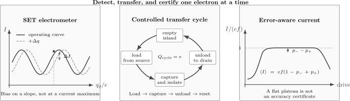
Detection, transfer, and certification are different layers. An SET electrometer is biased on the slope of a Coulomb oscillation so an induced charge produces an output change. A pump cycle loads, captures, unloads, and resets an island. An ideal plateau has $\langle I\rangle=ef$, but missed and extra transfers shift it to $ef(1-p_-+p_+)$; plateau flatness alone does not determine either probability.

Single-Electron Transistor

From Coulomb oscillation to transducer

A normal single-electron transistor has an island between source and drain tunnel junctions and a capacitively coupled gate. The gate changes the dimensionless offset charge

$$n_g = \frac{C_gV_g+Q_0+\cdots}{e},$$

and the current repeats ideally when $n_g$ advances by one. The static charge-state derivation and gate period

$$\Delta V_g = \frac{e}{C_g}$$

are developed in Coulomb Blockade.

For sensing, the SET is operated on a flank of a Coulomb peak. A small induced charge $\delta q_{\mathrm{ind}}$ changes the output current by

$$\delta I \simeq \frac{\partial I}{\partial q_g} \delta q_{\mathrm{ind}},$$

where

$$q_g \equiv C_gV_g+Q_0+\cdots.$$

At the current maximum,

$$\frac{\partial I}{\partial q_g} = 0,$$

so maximum current is generally not maximum small-signal charge responsivity. The chosen operating point balances slope, output noise, dissipation, linear range, and backaction.

An input-referred charge-noise spectral density is

$$S_q(\omega) = \frac{ S_I(\omega) }{ \left| \partial I/\partial q_g \right|^2 },$$

provided one output quadrature and a locally linear response are being used. Charge sensitivity is usually reported as

$$q_n(\omega) \equiv \sqrt{S_q(\omega)}$$

in units such as $e/\sqrt{\mathrm{Hz}}$. A sensitivity number is incomplete without the analysis frequency, bandwidth, operating point, and spectral-density convention.

Radio-frequency operation

A dc SET often has a large resistance. Combined with cable and amplifier capacitance, that resistance can make direct readout slow. In an RF-SET, the device is embedded in an impedance-matching resonator. Charge-dependent SET impedance changes the amplitude and phase of a reflected carrier.

For a resonator with center frequency $f_0$ and loaded quality factor $Q_L$, a useful order-of-magnitude bandwidth is

$$B_{\mathrm{res}} \sim \frac{f_0}{Q_L}.$$

This is not necessarily the full measurement bandwidth. Coupling, amplifier noise temperature, nonlinear response, demodulation filters, and the SET’s own dynamics can be more restrictive.

RF readout moves the measurement away from low-frequency amplifier noise and can support time-resolved tunneling. It does not remove SET charge noise, shot noise, heating, or detector backaction.

Charge Sensing

Coupling a target to a detector

Let a target island with occupation $N$ be capacitively coupled to a detector. One target-electron transition shifts the detector’s effective input charge by

$$\Delta q_{\mathrm{det}} = \lambda e,$$

where the dimensionless coupling $\lambda$ depends on the mutual capacitance and the complete capacitance network. The detector signal step is

$$\Delta y \simeq \frac{\partial y}{\partial q_{\mathrm{det}}} \lambda e,$$

with $y$ an output current or reflected quadrature.

A clear detector step answers an electrostatic question: the target charge changed. It does not identify spin directly. Spin readout first converts spin information into a charge outcome through an energy-selective or Pauli-selective process. Spin Qubits owns that conversion and its fidelity ledger.

Averaged detection and single-shot detection

Two charge states with output means $y_0$ and $y_1$ are distinguishable only relative to their distributions. Define

$$\Delta y = \left| y_1-y_0 \right|.$$

If white input-referred charge noise has one-sided amplitude $q_n$, ideal rectangular averaging for duration $\tau$ gives the scale

$$\sigma_q(\tau) \simeq \frac{q_n}{\sqrt{2\tau}}.$$

The corresponding idealized signal-to-noise ratio is

$$\mathrm{SNR} \simeq \frac{ \Delta q_{\mathrm{det}} \sqrt{2\tau} }{ q_n }.$$

Real single-shot fidelity also depends on state relaxation during integration, detector ring-up, threshold choice, non-Gaussian noise, and prior probabilities. Integrating longer eventually stops helping when the target state changes or low-frequency drift dominates.

Event counting

A two-state target often produces a random-telegraph record. If its loading and unloading rates are $\gamma_{\mathrm{in}}$ and $\gamma_{\mathrm{out}}$, the ideal dwell-time densities are

$$p_{\mathrm{empty}}(t) = \gamma_{\mathrm{in}} \exp \left( -\gamma_{\mathrm{in}}t \right),$$

and

$$p_{\mathrm{occupied}}(t) = \gamma_{\mathrm{out}} \exp \left( -\gamma_{\mathrm{out}}t \right).$$

Finite detector bandwidth rounds steps and hides short dwells. A thresholded event list is trustworthy only when detector response and missed-event corrections are included. Hidden-Markov or likelihood methods can use the analog record more efficiently, but they still require a validated detector model.

The detector also perturbs the target. Bias-driven charge fluctuations can induce transitions, broaden levels, heat reservoirs, or dephase coherent superpositions. A noninvasive label means weak enough for a stated observable and timescale, not zero coupling.

Detector	Strength	Common limitation
SET electrometer	large charge gain and RF compatibility	periodic response, offset-charge drift, dissipation
QPC detector	simple gate-defined integration near semiconductor dots	shot-noise backaction and conductance drift
gate or dispersive sensor	low direct dc current through target	resonator calibration and state-dependent quantum capacitance
transport through target	direct current observable	invasive and blind to blocked or very slow events

Pumps and Turnstiles

Pump, turnstile, and source

A pump uses a periodic control cycle to transfer a net charge, potentially at zero average source–drain bias. A turnstile usually combines a directional bias with time-dependent barriers or gate charge so loading and unloading occur in a prescribed order. A dynamic quantum-dot source can instead capture carriers and emit them on demand into a conductor.

These names describe protocols, not sharply disjoint Hamiltonians. The operational distinction is the sequence of allowed transitions.

For one electron per period $T=1/f$, an ideal four-stage cycle is:

1. load: lower the source barrier or addition threshold so one electron enters;
2. capture: close the source side while keeping the desired charge state bound;
3. unload: open the drain side or raise the level so the electron exits;
4. reset: return the empty island to its initial control point.

The time-scale requirements include

$$\int_{\mathrm{load}} \gamma_{\mathrm{in}}(t)\,dt \gg 1,$$ $$\int_{\mathrm{unload}} \gamma_{\mathrm{out}}(t)\,dt \gg 1,$$

and, for every unwanted route,

$$\int_{\mathrm{cycle}} \gamma_{\mathrm{err}}(t)\,dt \ll 1.$$

For constant loading rate over a window $\tau_L$, the missed-loading probability is

$$P_{\mathrm{miss}} = \exp \left( -\gamma_{\mathrm{in}}\tau_L \right).$$

Slower driving suppresses missed events but can increase leakage, backtunneling, or thermal errors. Faster driving increases current but can create nonadiabatic excitations and incomplete capture. There is no universal instruction to drive as slowly or as quickly as possible.

Two-gate pump cycle

In a multi-island pump, two phase-shifted gates trace a closed path through a charge-stability diagram. A loop around a suitable degeneracy transfers an integer charge when each boundary crossing activates the intended junction in sequence. Reversing the loop orientation reverses the current.

This integer transfer is not automatically topological. Ordinary metallic and semiconductor pumps can depend continuously on barrier rates, waveform shape, and thermal occupation. Robust plateaus arise from protected timing and energetics, not necessarily from a Chern number.

Dynamic capture

In a tunable-barrier quantum-dot pump, the entrance barrier rises while the dot potential changes. Several electrons may load initially; unwanted electrons then backtunnel until a final charge state is isolated. Decay-cascade models describe the resulting capture probabilities. Waveform shaping can separate the desired loading and backtunneling stages and improve plateau flatness.

Model agreement is useful for optimization, but metrological accuracy cannot be assigned from a fit alone. A direct comparison or validated error-counting method is needed.

Metrology

Quantized-current relation

If exactly $n$ electrons cross a section in each cycle at frequency $f$, the average current magnitude is

$$I = nef.$$

For one electron per cycle,

$$I = ef.$$

At

$$f = 1.000\ \mathrm{GHz},$$

the exact elementary-charge value gives

$$I = 160.2176634\ \mathrm{pA}.$$

Producing $1.00\ \mathrm{nA}$ with one electron per cycle would require

$$f \simeq 6.24\ \mathrm{GHz}.$$

This exposes the central engineering tension: useful current favors high frequency or parallel channels, whereas accuracy favors enough time and energy selectivity to reject wrong transfers.

Error probabilities and current

Suppose the intended transfer is one electron. Let $p_-$ be the probability of a missing transfer and $p_+$ the probability of one extra transfer, with higher multiplicities negligible. Then

$$\frac{ \langle Q\rangle }{e} = 1-p_-+p_+,$$

and

$$\langle I\rangle = ef \left( 1-p_-+p_+ \right).$$

The relative current error is

$$\varepsilon_I \equiv \frac{ \langle I\rangle-ef }{ef} = p_+-p_-.$$

The mean current is sensitive to the difference of error probabilities. For independent rare errors, the low-frequency one-sided current-noise scale is instead

$$S_I(0) \simeq 2e^2f \left( p_-+p_+ \right).$$

Mean and noise therefore constrain different combinations. Opposite-sign errors can cancel in the mean while still producing excess fluctuations.

Ampere realization

Since 20 May 2019, the SI fixes

$$e = 1.602176634\times10^{-19}\ \mathrm{C}$$

exactly. A frequency-referenced electron pump is therefore conceptually direct: count elementary charges per SI second. The BIPM’s mise en pratique lists single-electron transport as one possible realization route while emphasizing that a practical realization needs a complete uncertainty statement.

The Josephson and quantum Hall effects provide a complementary electrical route:

$$V_J = n_J \frac{h f_J}{2e},$$ $$R_H = \frac{h}{i e^2}.$$

Ohm’s law then gives

$$\frac{V_J}{R_H} = \frac{ n_J i }{2} e f_J.$$

Comparing that current with a pump current $n_pef_p$ closes a quantum metrology triangle. Because $e$ and $h$ now have exact SI values, such comparisons test consistency of practical realizations and device corrections rather than determining those constants from scratch.

What constitutes an accuracy claim?

A metrological claim needs more than an apparent plateau:

1. traceability of frequency, current gain, resistance, and voltage references;
2. type-A statistical and type-B systematic uncertainty components;
3. tests versus frequency, temperature, drive amplitude, waveform, bias, and magnetic field where relevant;
4. reversal or null protocols that expose offsets;
5. a model or direct count of missed, extra, leakage, and higher-order events;
6. stability over the averaging interval;
7. a declared coverage factor and confidence interpretation.

A model-extrapolated error estimate, a plateau slope, and a directly measured uncertainty are different statements and should be labeled accordingly.

Practical Limitations

Error budget

Error channel	Mechanism	Leading diagnostic or mitigation
missed loading or unloading	finite rate during an open window	lengthen or reshape window; measure dwell-rate dependence
backtunneling	captured electron escapes to source	raise entrance barrier faster or improve energy selectivity
thermal activation	reservoir supplies an uphill transition	lower electron temperature; increase protection energy
cotunneling	higher-order virtual transfer bypasses sequence	increase barrier resistance; add junctions; test coupling scaling
photon-assisted tunneling	environment supplies energy	filtering, shielding, impedance control
nonadiabatic excitation	drive populates unwanted states	waveform shaping and excitation spectroscopy
Andreev transfer	two electrons cross an NS interface coherently	charging-energy and gap engineering; bias selection
quasiparticle poisoning	nonequilibrium quasiparticle changes parity	traps, shielding, thermalization, parity monitoring
offset-charge drift	fluctuators shift operating point	feedback, differential protocols, materials control
reservoir heating	dissipated power broadens occupations	reduce power, improve thermal anchoring, pulse duty cycle
detector undercount	events occur faster than detector response	bandwidth calibration and missed-event inference
leakage path	unintended island or parallel conduction	gate maps, bias dependence, device redesign

Proximity and Andreev Physics owns normal–superconductor interface amplitudes, Andreev reflection, and hybrid bound states. Here those processes appear only as entries in a hybrid-turnstile error budget.

Stability, bandwidth, and backaction

Increasing detector bias generally improves output signal but also increases shot noise and dissipation. Increasing resonator bandwidth lowers ring-up time but can reduce impedance transformation or sensitivity. Increasing mutual capacitance strengthens the signal but also the electrostatic perturbation.

These tradeoffs are summarized schematically by

$$\text{measurement rate} \longleftrightarrow \text{backaction rate},$$

not by a universal equality. Quantum-limited relations require a specified detector model and measured noise correlations.

Low-frequency charge noise deserves its own audit. A single fluctuator produces random-telegraph switching; a broad distribution of switching times can produce an approximate $1/f$ spectrum. One-over-f Noise owns that ensemble logic and the limits of spectral inference.

Scalability and operating temperature

Room-temperature single-electron operation requires charging and confinement energies well above $k_BT$, which pushes dimensions and capacitances downward. Fabrication variability, background charges, contact resistance, and readout then become more severe. Demonstrating one room-temperature Coulomb feature does not establish a reproducible logic or metrology platform.

Large arrays introduce wiring, calibration, cross-capacitance, fan-out, and heat-load constraints. A single-electron transistor can exhibit current gain in a circuit, but a periodic transfer curve and high output impedance do not automatically supply the voltage gain, noise margin, and power gain required by a scalable logic family.

Common Mistakes

1. Equating Coulomb oscillations with single-electron accuracy. Oscillations establish charge sensitivity, not one-error-per-cycle performance.
2. Biasing at the peak instead of the slope. Peak current can have zero first-order charge responsivity.
3. Reporting charge sensitivity without frequency or bandwidth. Low-frequency drift and white-noise performance can differ by orders of magnitude.
4. Treating thresholded events as ground truth. Finite response hides short dwells and merges rapid transitions.
5. Calling every frequency-locked plateau quantized. Leakage and opposite-sign errors can leave a deceptively flat mean.
6. Assuming slower drive is always better. It can increase backtunneling and thermal exposure.
7. Calling an ordinary pump topological. Integer transfer alone does not imply a topological invariant.
8. Using $I=ef$ without an uncertainty budget. The equation is exact only when the transfer count is exact.
9. Treating post-2019 metrology as a measurement of $e$. The SI fixes $e$; experiments realize and compare units.
10. Ignoring detector backaction. Resolving an event requires coupling that can alter the event statistics.

Exercises

1. Input-referred charge sensitivity

An SET has current slope

$$\left| \frac{\partial I}{\partial q_g} \right| = 8.0\ \mathrm{nA}/e$$

and white output-current noise

$$\sqrt{S_I} = 20\ \mathrm{fA}/\sqrt{\mathrm{Hz}}.$$

Find its input-referred charge sensitivity. Under the ideal white-noise averaging convention used above, estimate the integration time for $\mathrm{SNR}=5$ on a signal $\Delta q=0.050e$.

Solution

The charge sensitivity is

$$\begin{aligned} q_n &= \frac{\sqrt{S_I}}{ \left| \partial I/\partial q_g \right| } \\ &= 2.5\times10^{-6} \frac{e}{\sqrt{\mathrm{Hz}}}. \end{aligned}$$

Using

$$\mathrm{SNR} = \frac{\Delta q\sqrt{2\tau}}{q_n},$$

gives

$$\begin{aligned} \tau &= \frac12 \left( \frac{ \mathrm{SNR}\,q_n }{ \Delta q } \right)^2 \\ &\simeq 3.1\times10^{-8}\ \mathrm s. \end{aligned}$$

The ideal estimate is about $31\ \mathrm{ns}$. Resonator ring-up, target relaxation, and nonwhite noise may require a longer practical integration.

2. Missed loading

A pump opens its entrance barrier for $1.0\ \mu\mathrm s$ with approximately constant loading rate $\gamma_{\mathrm{in}}=5.0\ \mathrm{MHz}$. Estimate the missed-loading probability.

Solution

For a Poisson loading process,

$$P_{\mathrm{miss}} = \exp \left( -\gamma_{\mathrm{in}}\tau_L \right).$$

Here

$$\gamma_{\mathrm{in}}\tau_L = 5.0,$$

so

$$P_{\mathrm{miss}} = e^{-5} \simeq 6.74\times10^{-3}.$$

This $0.674\%$ error is far too large for precision current generation even though loading succeeds on most cycles.

3. Quantized current

Find the ideal current for a pump transferring three electrons per cycle at $f=500\ \mathrm{MHz}$.

Solution

Use

$$I = nef.$$

Then

$$\begin{aligned} I &= 3 \left( 1.602176634\times10^{-19}\ \mathrm C \right) \left( 5.00\times10^8\ \mathrm{s^{-1}} \right) \\ &\simeq 2.4033\times10^{-10}\ \mathrm A \\ &= 240.33\ \mathrm{pA}. \end{aligned}$$

4. Opposite-sign transfer errors

A one-electron pump has missed-transfer probability $p_-=2.0\ \mathrm{ppm}$ and extra-transfer probability $p_+=0.50\ \mathrm{ppm}$. Find the relative mean-current error. Why does a small mean error not imply a small total error rate?

Solution

The relative mean error is

$$\varepsilon_I = p_+-p_- = -1.50\ \mathrm{ppm}.$$

The total probability of a wrong cycle is approximately

$$p_-+p_+ = 2.50\ \mathrm{ppm}.$$

Mean current measures the signed difference, whereas error counts and low-frequency noise depend mainly on the sum. Opposite errors can partially cancel in the mean.

5. Frequency needed for one nanoampere

What drive frequency gives $1.00\ \mathrm{nA}$ for an ideal one-electron-per-cycle pump?

Solution

Solve

$$f = \frac{I}{e}.$$

Therefore

$$\begin{aligned} f &= \frac{ 1.00\times10^{-9}\ \mathrm A }{ 1.602176634\times10^{-19}\ \mathrm C } \\ &\simeq 6.24\times10^9\ \mathrm{Hz}. \end{aligned}$$

The required frequency is about $6.24\ \mathrm{GHz}$, illustrating why parallelization or multiple-electron transfer can be attractive and why bandwidth errors matter.

6. Reverse the pump

A two-gate pump transfers one electron from source to drain when its control trajectory encircles a charge degeneracy clockwise. What happens if the phase relation is reversed so the same loop is traversed counterclockwise, assuming all intended transitions remain adiabatically ordered?

Solution

The sequence of boundary crossings reverses: the device loads from the former drain and unloads toward the former source. The pumped charge changes sign,

$$Q_{\mathrm{cycle}} \mapsto -Q_{\mathrm{cycle}},$$

so the dc current reverses. Direction reversal is a valuable control because many offsets and leakage currents do not reverse in the same way.

7. Plateau versus accuracy

An experiment observes a current plateau whose slope versus gate amplitude is consistent with zero within measurement noise. List three reasons this does not establish $I=ef$ at a stated relative uncertainty.

Solution

Any three of the following are sufficient:

• a constant missed-transfer probability can shift the entire flat plateau;
• extra and missing transfers can cancel in the mean;
• current-gain or offset calibration can be wrong;
• leakage can be independent of gate amplitude over the tested interval;
• the frequency reference or waveform at the device may be miscalibrated;
• finite detector bandwidth can hide errors;
• the tested temperature, bias, or frequency range may not expose the dominant mechanism;
• no type-B systematic uncertainty budget has been supplied.

Plateau flatness is a robustness diagnostic, not an accuracy certificate.

8. Quantum metrology triangle

A Josephson array operates on index $n_J$ at frequency $f_J$, a quantum Hall device is on integer plateau $i$, and a pump transfers $n_p$ electrons at frequency $f_p$. Derive the ideal closure condition obtained by comparing the pump current with $V_J/R_H$.

Solution

The Josephson and Hall relations give

$$\frac{V_J}{R_H} = \frac{ n_J i }{2} e f_J.$$

The pump gives

$$I_p = n_p e f_p.$$

Equating the currents and canceling $e$ gives

$$n_p f_p = \frac{ n_J i }{2} f_J.$$

Equivalently, the closure ratio

$$\mathcal K \equiv \frac{ 2n_pf_p }{ n_J i f_J }$$

should equal one after all realization corrections and uncertainties are included.

Connections

• Coulomb Blockade derives the charge-state energies, tunnel-junction criteria, diamond slopes, and static SET operating principle.
• Quantum Point Contacts develops QPC charge responsivity, time resolution, detector backaction, and spin-to-charge readout context.
• Quantum Dots supplies confined orbitals, addition spectra, and tunable barriers for semiconductor pumps and sensed targets.
• Proximity and Andreev Physics develops the normal–superconductor conversion processes that enter hybrid turnstiles as intended pair transfer or as an error channel.
• Mesoscopic Transport derives jump-process currents, waiting times, shot noise, and full counting statistics.
• Spin Qubits owns state preparation, spin-to-charge conversion, Pauli blockade, readout fidelity, and relaxation.
• One-over-f Noise explains random-telegraph fluctuators and broad switching-rate ensembles.
• Fundamental Constants explains exact defining constants, adjusted constants, and uncertainty propagation after the SI redefinition.
• Josephson Effect supplies the voltage–frequency relation used in quantum electrical metrology.
• Integer Quantum Hall Effect supplies the quantized Hall resistance and its metrological conditions.
• Nanostructures for Quantum Technology extends the transfer-error ledger to process yield, calibration, cryogenic infrastructure, and task-level evidence.
• Conventions for Quantum Matter fixes current direction, electron charge, and spectral-density conventions.

References

1. M. A. Kastner, “The Single-Electron Transistor,” Reviews of Modern Physics 64, 849–858 (1992), doi:10.1103/RevModPhys.64.849.
2. K. K. Likharev, “Single-Electron Devices and Their Applications,” Proceedings of the IEEE 87, 606–632 (1999), doi:10.1109/5.752518.
3. R. J. Schoelkopf, P. Wahlgren, A. A. Kozhevnikov, P. Delsing, and D. E. Prober, “The Radio-Frequency Single-Electron Transistor (RF-SET): A Fast and Ultrasensitive Electrometer,” Science 280, 1238–1242 (1998), doi:10.1126/science.280.5367.1238.
4. M. Field, C. G. Smith, M. Pepper, D. A. Ritchie, J. E. F. Frost, G. A. C. Jones, and D. G. Hasko, “Measurements of Coulomb Blockade with a Noninvasive Voltage Probe,” Physical Review Letters 70, 1311–1314 (1993), doi:10.1103/PhysRevLett.70.1311.
5. W. Lu, Z. Ji, L. Pfeiffer, K. W. West, and A. J. Rimberg, “Real-Time Detection of Electron Tunnelling in a Quantum Dot,” Nature 423, 422–425 (2003), doi:10.1038/nature01642.
6. S. Gustavsson et al., “Counting Statistics of Single-Electron Transport in a Quantum Dot,” Physical Review Letters 96, 076605 (2006), doi:10.1103/PhysRevLett.96.076605.
7. L. J. Geerligs, V. F. Anderegg, P. A. M. Holweg, J. E. Mooij, H. Pothier, D. Esteve, C. Urbina, and M. H. Devoret, “Frequency-Locked Turnstile Device for Single Electrons,” Physical Review Letters 64, 2691–2694 (1990), doi:10.1103/PhysRevLett.64.2691.
8. L. P. Kouwenhoven, A. T. Johnson, N. C. van der Vaart, C. J. P. M. Harmans, and C. T. Foxon, “Quantized Current in a Quantum-Dot Turnstile Using Oscillating Tunnel Barriers,” Physical Review Letters 67, 1626–1629 (1991), doi:10.1103/PhysRevLett.67.1626.
9. H. Pothier, P. Lafarge, C. Urbina, D. Esteve, and M. H. Devoret, “Single-Electron Pump Based on Charging Effects,” Europhysics Letters 17, 249–254 (1992), doi:10.1209/0295-5075/17/3/011.
10. J. P. Pekola, J. J. Vartiainen, M. Möttönen, O.-P. Saira, M. Meschke, and D. V. Averin, “Hybrid Single-Electron Transistor as a Source of Quantized Electric Current,” Nature Physics 4, 120–124 (2008), doi:10.1038/nphys808.
11. V. Kashcheyevs and B. Kaestner, “Universal Decay Cascade Model for Dynamic Quantum Dot Initialization,” Physical Review Letters 104, 186805 (2010), doi:10.1103/PhysRevLett.104.186805.
12. S. P. Giblin et al., “Towards a Quantum Representation of the Ampere Using Single Electron Pumps,” Nature Communications 3, 930 (2012), doi:10.1038/ncomms1935.
13. J. P. Pekola, O.-P. Saira, V. F. Maisi, A. Kemppinen, M. Möttönen, Y. A. Pashkin, and D. V. Averin, “Single-Electron Current Sources: Toward a Refined Definition of the Ampere,” Reviews of Modern Physics 85, 1421–1472 (2013), doi:10.1103/RevModPhys.85.1421.
14. M. W. Keller, A. L. Eichenberger, J. M. Martinis, and N. M. Zimmerman, “A Capacitance Standard Based on Counting Electrons,” Science 285, 1706–1709 (1999), doi:10.1126/science.285.5434.1706.
15. Bureau International des Poids et Mesures, “Mise en pratique for the definition of the ampere and other electrical units in the SI,” SI Brochure, 9th ed., Appendix 2 (2019), BIPM publication.

Further reading

• M. H. Devoret, D. Esteve, and C. Urbina, “Single-Electron Transfer in Metallic Nanostructures,” Nature 360, 547–553 (1992), doi:10.1038/360547a0.
• A. A. Clerk, M. H. Devoret, S. M. Girvin, F. Marquardt, and R. J. Schoelkopf, “Introduction to Quantum Noise, Measurement, and Amplification,” Reviews of Modern Physics 82, 1155–1208 (2010), doi:10.1103/RevModPhys.82.1155.