Quantum Wires

A quantum wire is an electronic system whose motion is quantized in two transverse directions but remains extended along one longitudinal direction. Its spectrum is therefore neither a three-dimensional continuum nor a fully discrete quantum-dot spectrum. Instead, each transverse eigenstate becomes a one-dimensional subband dispersing with longitudinal wavevector.

That definition is spectral, not merely geometric. A narrow fabricated object can contain hundreds of unresolved transverse modes and behave semiclassically. Conversely, an electrostatically defined channel inside a two-dimensional electron gas can be a clean quantum wire even though no freestanding wire is visible.

This page is the canonical home for transverse quantization, wire subbands, Fermi-point counting, the noninteracting one-dimensional density of states, and the boundary between a wire, a point contact, and a dot. Quantum Point Contacts owns short gate-defined bottlenecks, local adiabatic modes, and charge-detector operation. Conductance Quantization owns the full Landauer plateau derivation and contact-resistance ledger. Quantum Coherence in Conductors owns dephasing and interference extraction. Luttinger Liquid Preview owns the interacting one-dimensional fixed point, bosonization, power-law correlations, and spin–charge separation.

Operational Definition

Let the wire run along $x$, with characteristic transverse widths $W_y$ and $W_z$. A useful quantum-wire hierarchy is

$$k_{\mathrm B}T,\, e\lvert V\rvert,\, \Gamma,\, \frac{\hbar}{\tau_{\mathrm{el}}} \ll \Delta_\perp,$$

where $\Delta_\perp$ is a relevant transverse subband spacing, $\Gamma$ is lifetime or contact broadening, and $\tau_{\mathrm{el}}$ characterizes elastic broadening. The inequalities need not be exact by orders of magnitude, but the transverse thresholds must be experimentally resolvable.

The wire is in the single-mode quantum limit when only its lowest orbital subband is occupied:

$$\varepsilon_1 < E_F < \varepsilon_2.$$

It is multimode quasi-one-dimensional when several transverse subbands are occupied while their mode structure remains resolved. Calling only the single-mode case “one-dimensional” is common in low-energy many-body theory; device physics often calls both regimes quantum wires and states the number of occupied modes separately.

Three classifications are independent:

Question	Relevant comparison	Possible answers
Is transverse motion quantized?	$\Delta_\perp$ versus $k_{\mathrm B}T$, $\Gamma$, and disorder broadening	unresolved, multimode, single-mode
Is longitudinal motion ballistic?	wire length $L$ versus transport mean free path $\ell_{\mathrm{tr}}$	ballistic, quasi-ballistic, diffusive, localized
Is phase retained?	path length versus $L_\phi$	coherent or dephased for the chosen observable

A wire can therefore be single-mode but incoherent, multimode but ballistic, or diffusive yet phase coherent. What Is Mesoscopic Physics? gives the full independent-scale ledger.

Effective-Mass Construction

Near a nondegenerate band extremum, a simple wire model is

$$H = -\frac{\hbar^2}{2m_x^\ast} \frac{\partial^2}{\partial x^2} + H_\perp,$$

with

$$H_\perp = -\frac{\hbar^2}{2m_y^\ast} \frac{\partial^2}{\partial y^2} - \frac{\hbar^2}{2m_z^\ast} \frac{\partial^2}{\partial z^2} + V_\perp(y,z).$$

Solve the transverse problem

$$H_\perp\chi_n(y,z) = \varepsilon_n\chi_n(y,z).$$

For a uniform wire, separation of variables gives

$$\Psi_{nk}(x,y,z) = \frac{e^{ikx}}{\sqrt L} \chi_n(y,z)$$

and

$$E_n(k) = \varepsilon_n + \frac{\hbar^2k^2}{2m_{x,n}^\ast}.$$

The index $n$ may stand for several transverse quantum numbers and internal labels. The longitudinal mass can depend on subband when the bulk band is nonparabolic or when confinement mixes bands. Effective Mass owns the approximation and its tensor form.

Rectangular hard-wall benchmark

For widths $W_y$ and $W_z$ with infinite barriers and an isotropic mass,

$$\chi_{n_y n_z}(y,z) = \frac{2}{\sqrt{W_yW_z}} \sin \left( \frac{n_y\pi y}{W_y} \right) \sin \left( \frac{n_z\pi z}{W_z} \right),$$

where $n_y,n_z=1,2,\ldots$, and

$$\varepsilon_{n_y n_z} = E_c + \frac{\hbar^2\pi^2}{2m^\ast} \left( \frac{n_y^2}{W_y^2} + \frac{n_z^2}{W_z^2} \right).$$

This is a scale-setting model, not a literal description of most gates. Finite barriers allow wavefunction leakage, smooth electrostatic confinement gives nonuniform level spacings, and charge rearrangement makes the potential density dependent.

In a split-gate wire made from a two-dimensional electron gas, the heterostructure has already quantized the vertical direction. One then solves a reduced lateral problem. For a parabolic lateral potential,

$$V(y) = \frac12m^\ast\omega_y^2y^2,$$

the lateral thresholds are

$$\varepsilon_n = \varepsilon_z + \hbar\omega_y \left( n+\frac12 \right), \qquad n=0,1,2,\ldots.$$

A GaAs scale estimate

Take a hard-wall lateral width $W=80\ \mathrm{nm}$ and $m^\ast=0.067m_e$. Relative to the fixed vertical mode,

$$\varepsilon_n^{(y)} = \frac{\hbar^2\pi^2n^2}{2m^\ast W^2}.$$

Numerically,

$$\varepsilon_1^{(y)} \approx 0.877\ \mathrm{meV}, \qquad \varepsilon_2^{(y)} \approx 3.51\ \mathrm{meV},$$

so

$$\Delta_{21} \approx 2.63\ \mathrm{meV}.$$

At $4.2\ \mathrm K$, $k_{\mathrm B}T\approx0.362\ \mathrm{meV}$, below this ideal spacing. That comparison makes resolved subbands plausible; it does not guarantee ballistic transport or unit transmission.

Local Modes in a Nonuniform Wire

Real wires vary along $x$. Define local transverse modes by

$$H_\perp(x)\chi_n(y,z;x) = \varepsilon_n(x)\chi_n(y,z;x)$$

and expand

$$\Psi(x,y,z) = \sum_n \phi_n(x) \chi_n(y,z;x).$$

Projection gives coupled longitudinal equations containing

$$P_{nm}(x) \equiv \left\langle \chi_n \middle| \partial_x\chi_m \right\rangle_\perp$$

and

$$Q_{nm}(x) \equiv \left\langle \chi_n \middle| \partial_x^2\chi_m \right\rangle_\perp.$$

The off-diagonal terms mix modes. A useful adiabatic condition is

$$\hbar v_x \left\lvert P_{nm} \right\rvert \ll \left\lvert \varepsilon_n-\varepsilon_m \right\rvert$$

for every relevant pair. Smooth confinement then lets a carrier follow one local transverse mode with little reflection. Abrupt gates, rough boundaries, impurities, and avoided crossings can violate this condition.

Subbands, Fermi Points, and Occupancy

For an even dispersion, every occupied subband contributes right- and left-moving Fermi points. In the parabolic model,

$$k_{F,n} = \frac{ \sqrt{ 2m_{x,n}^\ast \left( E_F-\varepsilon_n \right) } }{\hbar}$$

when $E_F>\varepsilon_n$. The corresponding speed is

$$v_{F,n} = \frac{\hbar k_{F,n}}{m_{x,n}^\ast}.$$

If $g_n$ counts spin, valley, or other unresolved degeneracy but not the two propagation directions, the zero-temperature line density is

$$n_{\mathrm{1D}} = \sum_{n:E_F>\varepsilon_n} \frac{g_nk_{F,n}}{\pi}.$$

Thus gate voltage does two things: it changes occupation within an existing subband and, when $E_F$ crosses a threshold, creates a new pair of Fermi points. The electrostatic gate lever arm need not be constant near a threshold because the density of states and screening change rapidly.

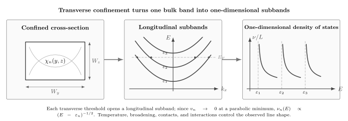
Two confined directions produce discrete transverse thresholds $\varepsilon_n$. Each threshold becomes a longitudinal subband $E_n(k_x)$, and each occupied even subband has right- and left-moving Fermi points. Because the group velocity vanishes at a parabolic band bottom, the ideal one-dimensional density of states diverges as $(E-\varepsilon_n)^{-1/2}$. Temperature, lifetime broadening, disorder, contacts, and interactions round or reconstruct the threshold.

One-Dimensional Density of States

For periodic length $L$, the allowed wavevectors are separated by

$$\Delta k = \frac{2\pi}{L}.$$

For a general subband, the density of states per unit length is

$$\frac{\nu_n(E)}{L} = \frac{g_n}{2\pi\hbar} \sum_{k_i:E_n(k_i)=E} \frac{1}{ \left\lvert v_n(k_i) \right\rvert },$$

where

$$v_n(k) = \frac{1}{\hbar} \frac{dE_n}{dk}.$$

For an even parabolic subband, the two roots $\pm k$ give

$$\frac{\nu_n(E)}{L} = \frac{g_n}{\pi\hbar} \sqrt{ \frac{m_{x,n}^\ast}{ 2 \left( E-\varepsilon_n \right) } } \, \Theta \left( E-\varepsilon_n \right).$$

Summing over $n$ produces a sequence of inverse-square-root van Hove singularities. Their origin is kinematic:

$$\frac{\nu_n(E)}{L} \propto \frac{1}{\lvert v_n(E)\rvert},$$

and $v_n\to0$ at a parabolic threshold.

The singularity is integrable

The ideal density of states diverges at $\varepsilon_n$, but the number of states in a small energy interval is finite:

$$\int_{\varepsilon_n}^{\varepsilon_n+\delta E} dE\, \frac{\nu_n(E)}{L} \propto \sqrt{\delta E}.$$

It is therefore wrong to interpret the divergence as an infinite carrier density. It means that many $k$ states are compressed into a small energy interval because the dispersion is flat near its minimum.

Thermal and lifetime rounding

An equilibrium probe samples a thermally weighted density of states. For example, the noninteracting quantum capacitance per unit length is

$$c_q(T) = e^2 \int dE\, \frac{\nu(E)}{L} \left( -\frac{\partial f}{\partial E} \right).$$

Finite lifetime, instrument resolution, density inhomogeneity, and subband-to-subband variation also round the ideal threshold. The measured electrochemical capacitance includes geometric electrostatics:

$$\frac{1}{c_\mu} = \frac{1}{c_g} + \frac{1}{c_q}$$

in a simple series model. Interactions replace the bare single-particle density of states by a thermodynamic compressibility and can invalidate this elementary decomposition.

Why a Density-of-States Peak Gives a Finite Conductance Step

The divergent density of states does not make the ideal conductance diverge. For one right-moving branch, the number of states in an interval $dE$ is

$$dN_{n,+} = L \frac{g_n}{2\pi\hbar v_n} dE.$$

Each state crosses a fixed section at rate $v_n/L$, so velocity cancels density of states:

$$\frac{v_n}{L} \frac{dN_{n,+}}{dE} = \frac{g_n}{h}.$$

With ideal reservoirs and elastic transmission, this cancellation leads to the familiar channel formula

$$G = \frac{e^2}{h} \sum_n g_n T_n(E_F).$$

When $T_n\approx1$, opening a spin-degenerate orbital mode adds approximately $2e^2/h$. The cancellation explains why a flat plateau can coexist with a sharply varying density of states.

This is only the bridge. Conductance Quantization owns finite-temperature Landauer transport, degeneracy conventions, bias spectroscopy, contact resistance, shot noise, and nonideal plateau diagnosis.

Wire, Point Contact, or Dot?

These terms describe different limits of the longitudinal problem.

Structure	Longitudinal character	Characteristic spectrum or measurement
extended quantum wire	approximately uniform over a length $L$	propagating subbands, possible 1D collective modes
quantum point contact	short constriction between wider reservoirs	local subband maxima and transmission steps
finite wire segment	reflections at two ends matter	Fabry–Pérot resonances or standing waves
quantum dot	escape is weak enough to resolve longitudinal levels and charging	discrete addition spectrum
geometric nanowire	structural label only	may be quantum, semiclassical, diffusive, or insulating

A point contact can be regarded as a short nonuniform quantum-wire segment, but its canonical observable is reservoir-to-reservoir transmission. A long wire supports internal propagation, distributed disorder, and interacting one-dimensional dynamics. If longitudinal confinement makes

$$\Delta_L \sim \frac{\pi\hbar v_F}{L}$$

larger than temperature and escape broadening, the same physical object acquires dot-like discrete levels. Quantum Dots owns that closed-island limit.

Spin, Valley, and Band Mixing

The integer $g_n$ must be measured or justified. It is not always two.

An in-plane magnetic field can approximately split a spinful subband as

$$E_{n,s}(k) = \varepsilon_n + \frac{\hbar^2k^2}{2m_n^\ast} + s \frac{g^\ast\mu_{\mathrm B}B}{2}, \qquad s=\pm1.$$

If the Zeeman splitting exceeds thermal and lifetime broadening, a nominal $2e^2/h$ step may resolve into two $e^2/h$ steps for ideal transmission. Orbital coupling, field-dependent confinement, exchange, and a density-dependent $g^\ast$ can complicate this picture.

Spin–orbit coupling can shift minima away from $k=0$, produce avoided crossings, and make spin expectation value depend on momentum. Valley degeneracy in silicon, carbon nanotubes, or multivalley semiconductors can be lifted by interfaces and confinement. Hole wires generally require a multiband valence-band Hamiltonian rather than one scalar effective mass. Spin–Orbit Coupling in Solids owns the material mechanisms.

The robust procedure is to count actual propagating branches at the Fermi energy and state which splittings the experiment resolves.

Interaction Bridge

The subband picture remains a necessary starting point, but one dimension amplifies interactions. Low-energy scattering is organized around a small set of Fermi points, screening is restricted, and a fermionic excitation can decay into collective density and spin waves.

For a clean, gapless, single-mode interacting wire, the generic low-energy description is a Tomonaga–Luttinger liquid. Consequences can include:

• separate charge and spin velocities;
• power-law tunneling density of states rather than a Fermi-liquid quasiparticle peak;
• interaction-dependent correlation exponents;
• strong sensitivity to a barrier or impurity;
• finite-size crossover when $\hbar v/L$ exceeds temperature or bias.

These statements do not mean that every narrow conductor has demonstrated a Luttinger liquid. A credible identification requires a controlled energy window and several linked observables, such as consistent tunneling exponents, excitation velocities, and finite-size scaling. Momentum-resolved tunneling between parallel semiconductor wires has directly probed dispersing collective excitations, while carbon-nanotube experiments have measured interaction-dependent power laws.

Two distinctions matter:

1. The noninteracting subband-edge law $\nu(E)\propto(E-\varepsilon_n)^{-1/2}$ is not the same object as the low-energy tunneling density of states of an interacting Luttinger liquid.
2. An ideal wire connected adiabatically to Fermi-liquid reservoirs can have reservoir-controlled two-terminal conductance even when its internal correlations are strong.

Luttinger Liquid Preview is the canonical continuation. It develops the harmonic-fluid Hamiltonian, the parameter $K$, bosonization, correlation exponents, spin–charge separation, impurities, and failure modes.

Physical Platforms

Platform	Source of transverse quantization	Important extra structure
split-gate semiconductor wire	vertical heterostructure plus lateral electrostatic gates	tunable width, smooth confinement, reservoir contacts
cleaved-edge wire	epitaxial confinement at an atomically defined edge	long clean channels and parallel-wire tunneling
freestanding semiconductor nanowire	finite cross-section and surface or interface potential	radial modes, facets, spin–orbit coupling, surface disorder
carbon nanotube	quantized circumferential crystal momentum	valley and spin degeneracy, curvature, strong interactions
epitaxial optical quantum wire	band offsets, strain, or self-assembled lateral confinement	electron–hole subbands and excitons
atomic chain or material edge	crystal and boundary electronic structure	lattice-scale bands; scalar effective mass may fail

An electronic edge state is one-dimensional in propagation but need not be a quantum wire in the confinement-subband sense used here. Chiral and helical boundary modes have additional symmetry or topology and belong to the corresponding topological pages.

Experimental Signatures

Gate and bias spectroscopy

Conductance steps locate subband openings only after contact transmission and degeneracy are controlled. A transconductance map,

$$\frac{\partial G}{\partial V_g},$$

often highlights threshold lines. Under finite source–drain bias, lines occur when a source or drain electrochemical potential crosses a subband edge. Their separations can estimate $\Delta_\perp$ and the gate lever arm.

Capacitance and compressibility

Capacitance can detect rapid changes in the thermodynamic density of states near subband thresholds. Geometric capacitance, parasitic channels, exchange-correlation contributions, and density-dependent confinement must be separated before identifying the ideal inverse-square-root law.

Momentum-resolved tunneling

Two parallel wires, or a wire adjacent to a two-dimensional layer, can exchange energy and momentum. Magnetic field can shift the relative momentum of tunneling states. The resulting resonance loci probe dispersions and, in interacting wires, collective spin and charge velocities.

Optical spectroscopy

Photoluminescence, absorption, and stimulated emission can reveal electron and hole subbands in epitaxial wires. Exciton binding, selection rules, strain, valence-band mixing, and disorder reshape the free-particle joint density of states, so an optical peak is not automatically a bare subband singularity.

Magnetic-field response

An in-plane field primarily tests Zeeman splitting, while a perpendicular field can alter orbital confinement and depopulate modes. Field orientation is therefore part of the model, not a secondary label.

Evidence Workflow

1. State the confinement geometry. Identify which two directions are quantized and whether the potential is hard-wall, electrostatic, radial, strain induced, or crystal specific.
2. Measure the threshold scale. Extract subband spacings from temperature, bias, capacitance, optical, or tunneling data rather than inferring them only from lithographic width.
3. Count occupied modes and degeneracies. Report spin, valley, and band labels separately.
4. Classify longitudinal transport. Compare $L$ with $\ell_{\mathrm{tr}}$, $L_\phi$, thermal length, and escape length.
5. Model contacts. Distinguish a uniform wire from a constriction and identify where voltage drops.
6. Test alternative threshold mechanisms. Resonant impurities, Coulomb blockade, localized states, and parallel channels can imitate steps or peaks.
7. Escalate interaction claims carefully. Require linked power laws, velocities, field response, or finite-size scaling rather than one anomalous plateau.

Common Mistakes

• Calling every fabricated nanowire a quantum wire without resolving transverse subbands.
• Treating “one-dimensional” as proof of single-mode occupancy.
• Confusing the transverse threshold $\varepsilon_n$ with a fully discrete energy level.
• Counting $\pm k$ as an extra internal degeneracy in $g_n$.
• Omitting spin or valley splitting while interpreting conductance-step size.
• Treating lithographic width as the electronic width of a depleted channel.
• Assuming a hard-wall potential when gates produce smooth, density-dependent confinement.
• Reading the ideal density-of-states divergence as an infinite carrier density.
• Expecting a density-of-states divergence in ideal conductance, despite velocity cancellation.
• Using a local bulk resistivity for a short ballistic constriction without a contact model.
• Calling a long interacting wire a noninteracting Landauer channel at every energy scale.
• Calling one power law definitive evidence of a Luttinger liquid.
• Confusing a topological edge channel with an ordinary confinement subband.
• Ignoring the crossover from a wire to a dot when longitudinal levels and charging become resolved.

Exercises

1. Hard-wall subband spacing

A lateral GaAs channel has $m^\ast=0.067m_e$ and hard-wall width $W=60\ \mathrm{nm}$. Find the first lateral energy and the spacing $\varepsilon_2-\varepsilon_1$.

Solution

For

$$\varepsilon_n = \frac{\hbar^2\pi^2n^2}{2m^\ast W^2},$$

using $\hbar^2/(2m_e)=38.10\ \mathrm{meV\,nm^2}$ gives

$$\varepsilon_1 = \frac{ \left( 38.10\ \mathrm{meV\,nm^2} \right) \pi^2 }{ 0.067 \left( 60\ \mathrm{nm} \right)^2 } \approx 1.56\ \mathrm{meV}.$$

Because $\varepsilon_2=4\varepsilon_1$,

$$\varepsilon_2-\varepsilon_1 = 3\varepsilon_1 \approx 4.68\ \mathrm{meV}.$$

A finite or smooth barrier changes both values and need not preserve the factor of four.

2. Density at the second-subband threshold

For a spin-degenerate hard-wall channel of width $W$, show that the line density just before the second lateral mode opens is $n_{\mathrm{1D}}=2\sqrt3/W$. Evaluate it for $W=80\ \mathrm{nm}$.

Solution

At the threshold,

$$E_F-\varepsilon_1 = \varepsilon_2-\varepsilon_1 = \frac{3\hbar^2\pi^2}{2m^\ast W^2}.$$

Therefore

$$k_{F,1} = \frac{\sqrt{2m^\ast(E_F-\varepsilon_1)}}{\hbar} = \frac{\sqrt3\pi}{W}.$$

With spin degeneracy $g=2$,

$$n_{\mathrm{1D}} = \frac{2k_{F,1}}{\pi} = \frac{2\sqrt3}{W}.$$

For $W=80\ \mathrm{nm}$,

$$n_{\mathrm{1D}} \approx 0.0433\ \mathrm{nm^{-1}} = 43.3\ \mu\mathrm m^{-1}.$$

3. Derive the parabolic one-dimensional density of states

Starting from one $k$ state per $2\pi/L$ and $E=\varepsilon+\hbar^2k^2/(2m^\ast)$, derive $\nu(E)/L$ for degeneracy $g$.

Solution

For $E>\varepsilon$, there are two roots $\pm k$. The state density per unit length and per $k$ is $g/(2\pi)$. Hence

$$\frac{\nu(E)}{L} = \frac{g}{2\pi} \sum_{\pm k} \left\lvert \frac{dk}{dE} \right\rvert.$$

Since

$$\frac{dE}{dk} = \frac{\hbar^2k}{m^\ast},$$

the two roots give

$$\frac{\nu(E)}{L} = \frac{g}{\pi} \frac{m^\ast}{\hbar^2\lvert k\rvert} = \frac{g}{\pi\hbar} \sqrt{ \frac{m^\ast}{2(E-\varepsilon)} }.$$

Multiplication by $\Theta(E-\varepsilon)$ enforces the threshold.

4. Integrability of the threshold

Show that the number of states per length between $\varepsilon$ and $\varepsilon+\delta E$ vanishes rather than diverges as $\delta E\to0^+$.

Solution

Write

$$\frac{\nu(E)}{L} = A \left( E-\varepsilon \right)^{-1/2}.$$

Then

$$\begin{aligned} \frac{\Delta N}{L} &= \int_\varepsilon^{\varepsilon+\delta E} dE\, \frac{\nu(E)}{L} \\ &= 2A \sqrt{\delta E}. \end{aligned}$$

The density of states is unbounded at one point, but its integral over a shrinking interval tends to zero as $\sqrt{\delta E}$.

5. Velocity–density-of-states cancellation

Explain why an ideal propagating mode contributes a finite conductance even though its density of states diverges at threshold.

Solution

For right movers, the number of states in a wire of length $L$ per energy is

$$\frac{dN_+}{dE} = L \frac{g}{2\pi\hbar v}.$$

Each occupied state crosses a section at frequency $v/L$. Their product is

$$\frac{v}{L} \frac{dN_+}{dE} = \frac{g}{2\pi\hbar} = \frac{g}{h}.$$

Thus the vanishing group velocity exactly cancels the divergent one-dimensional density of states. Reservoir occupation imbalance then produces $G=ge^2/h$ for unit transmission.

6. Adiabaticity test

A wire changes width over a scale $\ell_{\mathrm{var}}$. Give a qualitative condition for negligible mixing between modes $n$ and $m$, and explain why an abrupt step is dangerous.

Solution

The local-mode coupling is controlled by

$$P_{nm} = \left\langle \chi_n \middle| \partial_x\chi_m \right\rangle_\perp,$$

which is typically of order $1/\ell_{\mathrm{var}}$ times a dimensionless overlap. Negligible mixing requires

$$\hbar v_x \left\lvert P_{nm} \right\rvert \ll \left\lvert \varepsilon_n-\varepsilon_m \right\rvert.$$

An abrupt step has large spatial derivatives, so it couples transverse modes and can reflect carriers even when both sides support propagating states.

7. Resolving spin

A wire has one occupied orbital mode. At zero field its spin degeneracy is unresolved; at high field the two spin thresholds separate and both transmissions remain near one. What plateau sequence is expected as gate voltage opens the branches?

Solution

At zero field the two spin branches open together, so the first ideal plateau is

$$G = \frac{2e^2}{h}.$$

When Zeeman splitting is resolved, one spin branch opens first:

$$G = \frac{e^2}{h},$$

followed by the second branch:

$$G = \frac{2e^2}{h}.$$

This interpretation requires orbital field effects, transmission changes, and interaction-induced splitting to be excluded or modeled.

8. Diagnose a threshold peak

A capacitance trace has a rounded peak where a conductance step appears. List five checks needed before identifying it with the ideal one-dimensional density of states.

Solution

Useful checks include: calibrating the gate lever arm; subtracting geometric and parasitic capacitance; verifying that peak width follows electron temperature or independently measured lifetime broadening; reproducing the threshold in finite-bias spectroscopy; ruling out a localized-state resonance or Coulomb blockade; testing magnetic splitting and degeneracy; checking density homogeneity along the wire; and comparing the inferred spacing with a self-consistent confinement model.

Agreement among conductance, bias, and capacitance scales is stronger evidence than the shape of one peak.

Connections

• Low-Dimensional Quantum Matter supplies the general confinement hierarchy, dimensional DOS pattern, infrared fluctuation logic, and crossover evidence that distinguish an effective one-dimensional regime.
• What Is Mesoscopic Physics? supplies the independent wavelength, mean-free-path, coherence, thermal, geometry, and contact scales.
• Quantum Coherence in Conductors distinguishes static scattering, dephasing, thermal averaging, and escape in longitudinal propagation.
• Universal Conductance Fluctuations derives the quasi-one-dimensional variance, $(L_\phi/L)^{3/2}$ scaling, and correlation-field estimate $B_cwL_\phi\sim h/e$.
• Quantum Point Contacts treats the short nonuniform limit, local adiabatic modes, split-gate electrostatics, and charge sensing.
• Conductance Quantization owns the Landauer formula, plateau diagnostics, contact resistance, degeneracy, finite bias, and shot noise.
• Quantum Dots treats the limit in which longitudinal confinement, charging, and weak escape produce a discrete addition spectrum.
• Quantum Wells treats the neighboring dimensional limit with one confined coordinate, two-dimensional subbands, constant DOS steps, and heterostructure optics.
• Low-Dimensional Quantum Gases compares dimensional state counting and thermodynamics across one, two, and three dimensions.
• Luttinger Liquid Preview develops the universal interacting one-dimensional theory, bosonization, power laws, and spin–charge separation.
• Fermi–Dirac Statistics supplies occupation factors and thermal smearing.
• Mesoscopic Transport develops reservoirs, rates, counting statistics, detector backaction, and explicit open-system descriptions.
• Condensed Matter Roadmap places quantum wires between the mesoscopic scale map and more specialized device and many-body topics.

Further Reading

• T. Ihn, Semiconductor Nanostructures: Quantum States and Electronic Transport, Oxford University Press (2009), doi:10.1093/acprof:oso/9780199534425.001.0001.
• S. Datta, Electronic Transport in Mesoscopic Systems, Cambridge University Press (1995), doi:10.1017/CBO9780511805776.
• Y. Imry, Introduction to Mesoscopic Physics, 2nd ed., Oxford University Press (2002), doi:10.1093/oso/9780198507383.001.0001.
• T. Giamarchi, Quantum Physics in One Dimension, Oxford University Press (2004), doi:10.1093/acprof:oso/9780198525004.001.0001.

References

1. H. Sakaki, “Scattering Suppression and High-Mobility Effect of Size-Quantized Electrons in Ultrafine Semiconductor Wire Structures,” Japanese Journal of Applied Physics 19, L735–L738 (1980), doi:10.1143/JJAP.19.L735.
2. B. J. van Wees et al., “Quantized Conductance of Point Contacts in a Two-Dimensional Electron Gas,” Physical Review Letters 60, 848–850 (1988), doi:10.1103/PhysRevLett.60.848.
3. D. A. Wharam et al., “One-Dimensional Transport and the Quantisation of the Ballistic Resistance,” Journal of Physics C: Solid State Physics 21, L209–L214 (1988), doi:10.1088/0022-3719/21/8/002.
4. K. Ismail, D. A. Antoniadis, and H. I. Smith, “One-Dimensional Subbands and Mobility Modulation in GaAs/AlGaAs Quantum Wires,” Applied Physics Letters 54, 1130–1132 (1989), doi:10.1063/1.100738.
5. C. W. J. Beenakker and H. van Houten, “Quantum Transport in Semiconductor Nanostructures,” Solid State Physics 44, 1–228 (1991), doi:10.1016/S0081-1947(08)60091-0.
6. S. Tarucha, T. Honda, and T. Saku, “Reduction of Quantized Conductance at Low Temperatures Observed in 2 to 10 $\mu$m-Long Quantum Wires,” Solid State Communications 94, 413–418 (1995), doi:10.1016/0038-1098(95)00102-6.
7. A. Yacoby, H. L. Stormer, N. S. Wingreen, L. N. Pfeiffer, K. W. Baldwin, and K. W. West, “Nonuniversal Conductance Quantization in Quantum Wires,” Physical Review Letters 77, 4612–4615 (1996), doi:10.1103/PhysRevLett.77.4612.
8. S. J. Tans et al., “Individual Single-Wall Carbon Nanotubes as Quantum Wires,” Nature 386, 474–477 (1997), doi:10.1038/386474a0.
9. F. D. M. Haldane, “‘Luttinger Liquid Theory’ of One-Dimensional Quantum Fluids. I,” Journal of Physics C: Solid State Physics 14, 2585–2609 (1981), doi:10.1088/0022-3719/14/19/010.
10. M. Bockrath et al., “Luttinger-Liquid Behaviour in Carbon Nanotubes,” Nature 397, 598–601 (1999), doi:10.1038/17569.
11. O. M. Auslaender, A. Yacoby, R. de Picciotto, K. W. Baldwin, L. N. Pfeiffer, and K. W. West, “Tunneling Spectroscopy of the Elementary Excitations in a One-Dimensional Wire,” Science 295, 825–828 (2002), doi:10.1126/science.1066266.
12. Y. Jompol et al., “Probing Spin–Charge Separation in a Tomonaga–Luttinger Liquid,” Science 325, 597–601 (2009), doi:10.1126/science.1171769.
13. D. L. Maslov and M. Stone, “Landauer Conductance of Luttinger Liquids with Leads,” Physical Review B 52, R5539–R5542 (1995), doi:10.1103/PhysRevB.52.R5539.
14. D. Gershoni et al., “Optical Transitions in Quantum Wires with Strain-Induced Lateral Confinement,” Physical Review Letters 65, 1631–1634 (1990), doi:10.1103/PhysRevLett.65.1631.