Quantum Coherence in Conductors

Quantum coherence in a conductor is the retention of relative phase information between electronic propagation amplitudes long enough for their interference to affect a measured quantity. Coherence is not the absence of scattering. Static elastic disorder can create a complicated network of paths while preserving their relative phases, so a conductor may be diffusive and coherent at the same time.

The operational questions are:

1. which path pairs contribute to the observable;
2. how their relative phase fluctuates in time and energy;
3. which length or time cuts off the interference;
4. how temperature, magnetic field, spin–orbit coupling, contacts, and fitting assumptions enter the extracted result.

This page is the canonical home for phase memory and its experimental extraction in normal conductors. It develops the dephasing functional, diffusive coherence length, representative microscopic mechanisms, low-temperature saturation problem, and the relation among weak localization, conductance fluctuations, and ring interference. What Is Mesoscopic Physics? owns the full scale hierarchy and thermal-versus-geometric regime map, Environment-Induced Decoherence owns the general reduced-state framework, and the later weak-localization and Aharonov–Bohm-ring pages own their complete transport derivations.

Operational Definition

Consider two alternatives whose unperturbed phase difference is $\phi_0$. A fluctuating scalar potential along a path $\mathbf r(t)$ contributes

$$\delta\phi(t) = -\frac{1}{\hbar} \int_0^t dt'\, \delta U \left( \mathbf r(t'),t' \right).$$

For two paths, $\delta U$ is replaced by the potential difference sampled by those paths. The phase-memory factor is

$$\mathcal C(t) \equiv \left\langle e^{i\delta\phi(t)} \right\rangle,$$

where the average may be over environmental dynamics, repeated measurements, electron energies, or disorder realizations, depending on the experiment.

If $\delta\phi$ is zero-mean Gaussian noise, the cumulant expansion terminates:

$$\mathcal C(t) = \exp \left[ -\frac12 \left\langle \delta\phi(t)^2 \right\rangle \right].$$

More generally one often writes

$$\left\lvert \mathcal C(t) \right\rvert = e^{-F(t)}$$

and defines a characteristic dephasing time by

$$F(\tau_\phi) = 1.$$

An exponential law $F(t)=t/\tau_\phi$ is a model, not the definition of coherence. Diffusive electron–electron dephasing, broad distributions of fluctuator times, and non-Markovian environments can produce stretched exponentials or other envelopes.

From time to length

In a ballistic path,

$$L_\phi^{\mathrm{bal}} \sim v_F\tau_\phi.$$

In a diffusive conductor,

$$L_\phi \equiv \sqrt{D\tau_\phi},$$

up to the convention used in the fitting function. Reporting $\tau_\phi$ without the diffusion constant, or $L_\phi$ without the model that defines it, loses essential information.

Coherence is observable dependent

A device does not possess one context-free coherence length. Different measurements weight different paths:

• weak localization emphasizes closed time-reversed loops;
• conductance fluctuations correlate a broad family of interfering paths;
• an Aharonov–Bohm ring selects paths with specified winding;
• a Fabry–Pérot cavity selects repeated reflections between interfaces;
• a resonance linewidth weights the dwell-time distribution and escape.

In a simple regime these extractions can agree on one $\tau_\phi$. Disagreement can reveal geometry, nonexponential decay, spin channels, thermal averaging, or a fitting model outside its range.

Static Disorder Versus Dephasing

Let the potential be decomposed schematically as

$$U(\mathbf r,t) = U_{\mathrm{static}}(\mathbf r) + \delta U(\mathbf r,t).$$

$U_{\mathrm{static}}$ changes elastic scattering amplitudes and path phases. If it is unchanged between measurements, it generates a reproducible interference fingerprint. The time-dependent part can transfer energy, entangle the electron with other degrees of freedom, or randomize phase between repetitions.

This distinction explains three facts that initially look contradictory:

1. a diffusive wire can undergo many elastic collisions and remain phase coherent;
2. two nominally identical disordered samples can have different conductance traces;
3. one sample can reproduce its trace until charge traps, impurities, or magnetic moments rearrange.

Elastic scattering reduces the transport mean free path. Dephasing limits phase-sensitive path duration. The corresponding times need not be close:

$$\tau_{\mathrm{tr}} \ll \tau_\phi$$

is common in low-temperature mesoscopic metals and semiconductors.

Diffusive Interference Modes

After averaging over static disorder, products of retarded and advanced propagators organize into long-lived diffusive modes. The Diffuson tracks probability propagation. The Cooperon tracks interference between a path and its time reverse and is especially sensitive to time-reversal breaking.

A schematic Cooperon channel has the form

$$\mathcal P_C \left( \mathbf q,\omega \right) \propto \frac{1}{ Dq^2 -i\omega + \tau_\phi^{-1} + \tau_B^{-1} + \tau_s^{-1} },$$

where $\tau_B$ represents orbital magnetic suppression and $\tau_s$ a magnetic or spin-channel relaxation rate. Spin–orbit coupling mixes singlet and triplet Cooperon channels rather than merely adding one scalar rate, so the displayed denominator is a structural guide.

The weak-localization correction contains an infrared-sensitive mode sum of the form

$$\delta\sigma_{\mathrm{int}} \propto -\frac{e^2D}{\hbar} \int \frac{d^dq}{(2\pi)^d} \frac{1}{ Dq^2+\tau_\phi^{-1}+\cdots }.$$

The elastic mean free path supplies an ultraviolet cutoff. $L_\phi$, sample size, magnetic field, spin relaxation, or escape supplies the infrared cutoff. The sign and prefactor depend on symmetry and channel multiplicity:

• constructive return from time-reversed paths lowers conductivity in the orthogonal class, giving weak localization;
• strong spin–orbit coupling can reverse the correction, giving weak antilocalization;
• magnetic scattering or orbital field suppresses the Cooperon.

The classical diffusion pole and the coherent correction are therefore not competing descriptions. The correction is built from coherent diffusion.

Microscopic Dephasing Mechanisms

The total electron-plus-environment state may evolve unitarily while a selected electronic amplitude loses visibility. Other electrons, phonons, magnetic moments, photons, detectors, and reservoirs can all carry away relative-phase information.

Mechanism	What records or randomizes phase?	Typical diagnostic issue
electron–electron interaction	electron–hole excitations and fluctuating screened fields	strongly dimension and disorder dependent
electron–phonon interaction	lattice excitations	power law depends on phonon spectrum and disorder
magnetic impurities	spin flips and Kondo dynamics	tiny concentrations can mimic saturation
external electromagnetic noise	fluctuating voltage or flux	can dephase before obvious dc heating
charge fluctuators	time-dependent electrostatic landscape	non-Gaussian and history-dependent noise
voltage probe or detector	which-path information and backaction	extraction apparatus changes the device
escape to reservoirs	loss of amplitude into equilibrating leads	limits dwell time but is not intrinsic bulk dephasing

When statistically independent mechanisms each produce exponential decay, one sometimes writes

$$\frac{1}{\tau_{\phi,\mathrm{eff}}} \approx \frac{1}{\tau_{ee}} + \frac{1}{\tau_{e\text{-}ph}} + \frac{1}{\tau_s} + \frac{1}{\tau_{\mathrm{env}}} + \frac{1}{\tau_{\mathrm{esc}}}.$$

This Matthiessen-like rule is phenomenological. Nonexponential kernels, coupled fluctuators, spin-channel matrices, and geometry-dependent escape can invalidate simple rate addition.

Electron–electron dephasing

Electron–electron interactions conserve the total energy and particle number of the isolated electron system, yet one quasiparticle can entangle with electron–hole excitations and lose single-particle phase memory. In diffusive conductors, small-energy-transfer scattering from fluctuating electromagnetic fields generated by the electrons themselves is often called Nyquist dephasing.

Representative equilibrium scalings in the diffusive Fermi-liquid regime are:

Effective dimension	Representative low-temperature scaling	Main caveat
quasi-one-dimensional	$\tau_\phi^{-1}\propto T^{2/3}$	requires transverse dimensions shorter than $L_\phi$ and $L_T$
two-dimensional	$\tau_\phi^{-1}\sim (k_{\mathrm B}T/\hbar g_\square)\ln g_\square$	$g_\square$ and screening vary with density and disorder
three-dimensional	$\tau_\phi^{-1}\propto T^{3/2}$	prefactor and crossover depend on disorder and screening

Here, in two dimensions,

$$g_\square \equiv \frac{\sigma_\square}{e^2/h}$$

is the dimensionless sheet conductance, up to the convention used for spin, valley, and other degeneracies. These exponents are not universal fits for ballistic, strongly localized, non-Fermi-liquid, or nonequilibrium conductors.

For a quasi-one-dimensional wire with approximately temperature-independent $D$,

$$\tau_\phi \propto T^{-2/3} \qquad \Longrightarrow \qquad L_\phi \propto T^{-1/3}.$$

The exponent on $L_\phi$ is half the exponent on $\tau_\phi$ because diffusion converts time to length through a square root.

Electron–phonon dephasing

Electron–phonon rates are often summarized as

$$\tau_{e\text{-}ph}^{-1} \propto T^p.$$

$p$ is not a material label. It depends on dimensionality, phonon polarization, disorder, screening, boundary conditions, and whether the phonons themselves are confined. A fitted power law over less than a decade rarely identifies the microscopic mechanism by itself.

Magnetic impurities

A dilute magnetic moment can flip electron spin and suppress time-reversed interference. Kondo screening makes the rate nonmonotonic in temperature and field. Extremely small impurity concentrations may produce an apparent plateau in $\tau_\phi(T)$ while leaving only a subtle signature in the ordinary resistance.

Noise and measurement backaction

External voltage noise can randomize phase even when the average injected power is small. A nearby quantum point contact or charge sensor can acquire which-path information. Filtering, grounding, lead impedance, detector bias, and microwave leakage are therefore part of a phase-coherence experiment, not merely laboratory details.

Low-Temperature Saturation

In an equilibrium, nonmagnetic diffusive Fermi liquid, phase space for electron–electron and electron–phonon scattering vanishes as $T\to0$. Standard theory therefore expects the intrinsic dephasing rate from these channels to approach zero, so $\tau_\phi$ grows until another scale limits the measurement.

Experiments have often reported an apparent low-temperature saturation:

$$\tau_\phi(T) \longrightarrow \tau_{\mathrm{sat}} \quad \text{as} \quad T\to0.$$

That observation is not a mechanism. Before claiming intrinsic zero-temperature dephasing, one must exclude:

• electron temperature saturating above the thermometer reading;
• microwave or radio-frequency noise;
• dilute magnetic impurities;
• two-level fluctuators;
• finite sample size, so $L_\phi$ has reached the device dimension;
• escape or dwell-time limits;
• fit insensitivity once the magnetoconductance feature becomes narrower than field resolution;
• an incorrect dimensionality or spin–orbit model.

The historical proposal that zero-point electromagnetic fluctuations produce a universal intrinsic saturation generated an important debate. Subsequent controlled experiments showed that magnetic impurities and source purity can account for saturation-like behavior in several metallic wires, while cleaner samples recover the expected quasi-one-dimensional $T^{-2/3}$ growth of $\tau_\phi$. The durable conclusion is methodological: a plateau in a fitted lifetime requires an experimental audit, not a universal interpretation.

Experimental Extractors

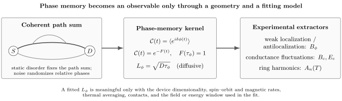
Phase coherence is inferred through a geometry and model. Static disorder fixes a reproducible path sum; dynamic fluctuations generate a coherence envelope $\mathcal C(t)$. Weak localization or antilocalization, conductance-correlation fields and energies, and Aharonov–Bohm harmonics weight different path families. Agreement among them is a stronger result than one unconstrained fit.

Weak localization and antilocalization

A small perpendicular field threads long diffusive loops and suppresses their time-reversed interference. In a common simplified two-dimensional convention,

$$\Delta\sigma(B) = \alpha \frac{e^2}{2\pi^2\hbar} \left[ \psi \left( \frac12 + \frac{B_\phi}{\lvert B\rvert} \right) - \ln \left( \frac{B_\phi}{\lvert B\rvert} \right) \right],$$

with

$$B_\phi = \frac{\hbar}{4eD\tau_\phi} = \frac{\hbar}{4eL_\phi^2}.$$

$\psi$ is the digamma function. The sign convention for $\alpha$ varies across the literature. Real fits may require separate elastic, spin–orbit, magnetic, intervalley, intersurface, or multiband fields. A good fit over a narrow interval does not establish that the single-channel formula is physically complete.

Weak localization averages over disorder and emphasizes time-reversed return paths. It can therefore remain visible even when sample-specific fluctuations have been smoothed by averaging.

Universal conductance fluctuations

Let

$$\delta G(B,E) = G(B,E) - \left\langle G \right\rangle.$$

A field correlation function can be defined by

$$C_B(\Delta B) = \left\langle \delta G(B) \delta G(B+\Delta B) \right\rangle_B.$$

The correlation field obeys an order-of-magnitude flux relation

$$B_cA_\phi \sim \frac{h}{e}.$$

For a two-dimensional coherent patch, $A_\phi\sim L_\phi^2$. In a narrow quasi-one-dimensional wire, the relevant loop area is often closer to $wL_\phi$, with geometry-dependent numerical factors. The energy correlation scale is of order

$$E_c \sim \frac{\hbar D}{L_{\mathrm{eff}}^2},$$

where $L_{\mathrm{eff}}$ is limited by $L$, $L_\phi$, or $L_T$ according to the measurement.

Aharonov–Bohm harmonics

For a ring with one-winding path length $P$, a simple coherence envelope gives

$$A_n(T) \sim A_n^{(0)} R_{T,n} \exp \left( -\frac{nP}{L_\phi} \right),$$

where $A_n$ is the $n$th $h/e$ harmonic and $R_{T,n}$ contains thermal averaging and geometry. Exact exponents differ between ballistic and diffusive rings and between canonical and grand-canonical conditions. The robust idea is that higher windings spend longer in the device and are more strongly suppressed.

Interferometers and resonances

Fabry–Pérot fringes, Mach–Zehnder visibility, resonant line shapes, and coherent charge oscillations can also constrain phase memory. Their contrast additionally depends on beam-splitter balance, contact transparency, mode mixing, energy averaging, and detector resolution. A declining visibility is not automatically a direct measurement of $\tau_\phi$.

Observable	Main path family	Useful scale	Frequent ambiguity
weak localization	time-reversed diffusive loops	$B_\phi$, $L_\phi$	spin–orbit, magnetic, intervalley, and interaction corrections
conductance fluctuations	sample-specific path pairs	$B_c$, $E_c$	background subtraction and thermal averaging
ring harmonics	fixed winding sectors	harmonic decay with $P$	area distribution and contact asymmetry
cavity fringes	repeated reflections	visibility and energy period	mode averaging and barrier drift
resonance linewidth	dwell-time distribution	$\Gamma\sim\hbar/\tau_{\mathrm{dwell}}$	escape broadening is not pure dephasing

Thermal Averaging and Nonequilibrium Bias

What Is Mesoscopic Physics? gives the canonical distinction. In linear response,

$$G(T) = \int dE\, \left( -\frac{\partial f}{\partial E} \right) G(E,0)$$

averages coherent patterns over an energy window of order $k_{\mathrm B}T$. At the same time, raising temperature can shorten $\tau_\phi$ microscopically. A fit should include both effects when

$$k_{\mathrm B}T \gtrsim E_c.$$

Finite source–drain bias adds further complications:

• the electronic distribution may become a double-step rather than a hotter Fermi function;
• Joule heating can make electron temperature exceed bath temperature;
• energy-dependent transmissions are sampled over $e\lvert V\rvert$;
• nonequilibrium electron–electron scattering can change the dephasing kernel;
• nonlinear conductance need not obey the simple two-terminal even-in-$B$ relation of linear response.

Replacing every finite-bias distribution by one effective temperature can hide the process one is trying to measure.

Effective Dimensionality

The dimension relevant to dephasing is the dimension explored by coherent diffusion.

A wire is quasi-one-dimensional for interference when its width $w$ and thickness $t$ satisfy

$$w,t \ll L_\phi,L_T,$$

even though its electrons occupy a three-dimensional band. A film is effectively two-dimensional when its thickness is shorter than the coherent diffusion lengths while its in-plane dimensions are larger. Dimensional crossover occurs as temperature changes $L_\phi$ and $L_T$.

This affects:

• the momentum integral of the Cooperon;
• the temperature exponent of electron–electron dephasing;
• the coherent area entering $B_c$;
• the magnetic-field orientation dependence;
• the fitting function for magnetoconductance.

Crystallographic dimension, electronic-subband dimension, and interference dimension should be stated separately.

Orbital, Spin, and Order-Parameter Coherence

$L_\phi$ from magnetotransport is primarily an orbital single-particle phase-memory length. It is not automatically:

• a spin relaxation length;
• a spin-echo $T_2$;
• an inhomogeneous spin dephasing time $T_2^\ast$;
• a charge-qubit coherence time;
• a superconducting coherence length;
• the phase stiffness of a condensate.

Spin–orbit coupling links orbital interference to spin rotation, which is why weak antilocalization can measure spin–orbit fields. The extracted parameters still depend on the spin-diffusion model. Decoherence Timescales owns the general $T_1$, $T_2$, and $T_2^\ast$ ledger, while Spin Qubits owns control and echo protocols.

Worked Diagnoses

Quasi-one-dimensional wire

Let

$$D = 0.020\ \mathrm{m^2\,s^{-1}}, \qquad \tau_\phi = 0.80\ \mathrm{ns}.$$

Then

$$\begin{aligned} L_\phi &= \sqrt{D\tau_\phi} \\ &= \sqrt{ \left( 0.020\ \mathrm{m^2\,s^{-1}} \right) \left( 0.80\times10^{-9}\ \mathrm s \right) } \\ &= 4.0\ \mu\mathrm m. \end{aligned}$$

For a $10\ \mu\mathrm m$ wire, the whole sample is not one coherent block. If its width is $w=120\ \mathrm{nm}$, the loop-area estimate

$$A_\phi \sim wL_\phi = 0.48\ \mu\mathrm m^2$$

gives

$$B_c \sim \frac{h/e}{A_\phi} \approx 8.6\ \mathrm{mT}.$$

The coefficient is geometry dependent, so this is a scale prediction rather than a precision extraction.

Two-dimensional magnetoconductance

Suppose a simplified fit gives

$$B_\phi = 2.0\ \mathrm{mT}.$$

Then

$$\begin{aligned} L_\phi &= \sqrt{ \frac{\hbar}{4eB_\phi} } \\ &\approx 0.287\ \mu\mathrm m. \end{aligned}$$

If $D=0.010\ \mathrm{m^2\,s^{-1}}$,

$$\tau_\phi = \frac{L_\phi^2}{D} \approx 8.2\ \mathrm{ps}.$$

These numbers are only as trustworthy as the dimensionality, field interval, classical-background subtraction, and spin-channel model.

Ring harmonics

For $P=3.0\ \mu\mathrm m$ and $L_\phi=2.0\ \mu\mathrm m$, the simple envelope predicts

$$\frac{A_2}{A_1} \sim \exp \left( -\frac{P}{L_\phi} \right) \approx 0.22,$$

before thermal and geometry-dependent prefactors. If the measured ratio is much larger, one should test whether $P$ is the correct path length, whether several areas contribute, or whether the assumed exponential kernel is inadequate.

Evidence Workflow

Establish the transport regime

State $D$, $\ell_{\mathrm{tr}}$, dimensions, density, and whether propagation is ballistic, diffusive, or localized. Do not fit a diffusive Cooperon to a device whose relevant path is shorter than the mean free path.

Establish electron temperature

Use an in situ thermometer when possible: Johnson noise, Coulomb-peak width, shot-noise crossover, or a calibrated resonance. Refrigerator temperature is a boundary condition, not a direct measurement of the electrons.

Choose the correct dimensionality

Compare $w$, $t$, $L_\phi$, and $L_T$ at every temperature. A crossover in fitted power law can be geometric rather than a new microscopic interaction.

Fit the full channel structure

Include spin–orbit, magnetic, intervalley, intersurface, or multiband channels when required. State the background model and field range. Report parameter covariance rather than only a best-fit $L_\phi$.

Cross-check observables

Compare weak-localization width, fluctuation correlation field, ring harmonics, and energy correlation where available. Their agreement in scale and temperature dependence is stronger evidence than one fit.

Audit saturation

Vary filtering, excitation current, detector bias, sample length, source purity, magnetic field, and cooldown. A lifetime plateau that moves under these controls is not an intrinsic zero-temperature constant.

Common Mistakes

• Calling a ballistic conductor coherent without measuring phase memory.
• Calling a diffusive conductor incoherent merely because it has many elastic collisions.
• Equating mobility with $L_\phi$.
• Assuming every coherence envelope is exponential.
• Adding dephasing rates when the underlying kernels or spin channels are coupled.
• Treating thermal averaging as phase destruction along one trajectory.
• Using the bath temperature when the electrons are overheated.
• Fitting a two-dimensional weak-antilocalization formula through a dimensional crossover.
• Treating the fitted prefactor $\alpha$ as a universal channel count.
• Ignoring classical magnetoresistance and interaction corrections in the fitting window.
• Using $B_cL_\phi^2=h/e$ in a narrow wire where the coherent area is closer to $wL_\phi$.
• Equating resonance escape width with pure dephasing.
• Equating orbital $L_\phi$ with spin $T_2$ or superconducting coherence length.
• Claiming intrinsic zero-temperature decoherence from one saturated curve.

Exercises

1. Gaussian phase noise

Show that zero-mean Gaussian phase noise gives $\mathcal C(t)=\exp[-\langle\delta\phi^2\rangle/2]$.

Solution

The cumulant expansion is

$$\ln \left\langle e^{i\delta\phi} \right\rangle = \sum_{n=1}^{\infty} \frac{i^n}{n!} \left\langle \delta\phi^n \right\rangle_c.$$

For zero-mean Gaussian noise, the first cumulant vanishes, the second is $\langle\delta\phi^2\rangle$, and every cumulant above second order is zero. Therefore

$$\ln\mathcal C = -\frac12 \left\langle \delta\phi^2 \right\rangle,$$

which gives the stated result. A non-Gaussian fluctuator generally produces higher cumulants and a different envelope.

2. Convert a dephasing time to length

A diffusive conductor has $D=0.015\ \mathrm{m^2\,s^{-1}}$ and $\tau_\phi=200\ \mathrm{ps}$. Find $L_\phi$.

Solution

$$\begin{aligned} L_\phi &= \sqrt{D\tau_\phi} \\ &= \sqrt{ \left( 0.015\ \mathrm{m^2\,s^{-1}} \right) \left( 2.00\times10^{-10}\ \mathrm s \right) } \\ &\approx 1.73\ \mu\mathrm m. \end{aligned}$$

Using $v_F\tau_\phi$ would be inappropriate because the motion is specified as diffusive.

3. Quasi-one-dimensional temperature scaling

If $\tau_\phi^{-1}\propto T^{2/3}$ and $D$ is temperature independent, how do $\tau_\phi$ and $L_\phi$ scale?

Solution

Inverting the rate gives

$$\tau_\phi \propto T^{-2/3}.$$

Since $L_\phi=\sqrt{D\tau_\phi}$,

$$L_\phi \propto T^{-1/3}.$$

A measured $L_\phi\propto T^{-2/3}$ would therefore not match this diffusive Nyquist prediction unless $D$ also had a strong temperature dependence or a different quantity was being fitted.

4. Coherence field

Use the simplified two-dimensional relation $B_\phi=\hbar/(4eL_\phi^2)$ to find $B_\phi$ for $L_\phi=0.50\ \mu\mathrm m$.

Solution

$$\begin{aligned} B_\phi &= \frac{\hbar}{4eL_\phi^2} \\ &= \frac{ 1.055\times10^{-34}\ \mathrm{J\,s} }{ 4 \left( 1.602\times10^{-19}\ \mathrm C \right) \left( 0.50\times10^{-6}\ \mathrm m \right)^2 } \\ &\approx 0.659\ \mathrm{mT}. \end{aligned}$$

This is a model parameter, not a universal field width for every device.

5. Correlation field in a narrow wire

A quasi-one-dimensional wire has $w=100\ \mathrm{nm}$ and $L_\phi=2.0\ \mu\mathrm m$. Estimate the conductance-fluctuation correlation field from $B_cwL_\phi\sim h/e$.

Solution

The coherent area estimate is

$$A_\phi \sim wL_\phi = 0.20\ \mu\mathrm m^2.$$

Therefore

$$\begin{aligned} B_c &\sim \frac{h/e}{A_\phi} \\ &\approx \frac{ 4.136\times10^{-15}\ \mathrm{T\,m^2} }{ 0.20\times10^{-12}\ \mathrm{m^2} } \\ &\approx 20.7\ \mathrm{mT}. \end{aligned}$$

Boundary conditions and the precise definition of correlation width change the numerical coefficient.

6. Static disorder test

Why does warming a sample enough to rearrange charge traps often change its conductance fingerprint even if its mobility after recooling is nearly unchanged?

Solution

Mobility summarizes momentum relaxation and can remain similar for two disorder configurations. The interference fingerprint depends on detailed path amplitudes and phases. Rearranged traps alter those phases, producing a new reproducible pattern after recooling. This is evidence that the original trace was sample-specific coherent interference rather than irreproducible measurement noise.

7. Audit a saturation claim

A fitted $\tau_\phi$ stops increasing below $80\ \mathrm{mK}$. List at least four controls required before calling this intrinsic zero-temperature dephasing.

Solution

Useful controls include an independent electron-temperature measurement; reducing excitation current and detector bias; improving microwave and radio-frequency filtering; comparing samples of different length; testing source purity or magnetic-impurity sensitivity; varying field to polarize magnetic moments; checking fit resolution and dimensionality; and comparing a second coherence observable such as fluctuation correlation or ring harmonics.

If the plateau tracks sample length, filtering, detector bias, cooldown, or impurity content, it is not a universal intrinsic constant.

8. Compare two coherence measurements

Weak-localization fitting gives $L_\phi=1.0\ \mu\mathrm m$, while ring harmonics suggest $2.0\ \mu\mathrm m$ in the same material. Give four possible reasons other than an arithmetic error.

Solution

The two devices may have different disorder or electron temperature; the observables weight different path-duration distributions; thermal averaging may have been included in only one analysis; spin–orbit, magnetic, or intervalley channels may make the weak-localization fit incomplete; contacts may add escape or detector backaction; the ring may contain several effective areas; or the coherence envelope may be nonexponential so no single $L_\phi$ describes both path families. Agreement is desirable, but disagreement is diagnostic rather than automatically contradictory.

Connections

• What Is Mesoscopic Physics? defines the independent confinement, scattering, phase, thermal, and contact scales used here.
• Environment-Induced Decoherence develops reduced states, environmental records, pointer structure, and the distinction between global unitarity and subsystem coherence.
• Decoherence Timescales distinguishes relaxation, homogeneous dephasing, inhomogeneous broadening, and echo times.
• Boltzmann Transport owns the collision-integral description of momentum and energy relaxation in the semiclassical bulk limit.
• Disorder in Quantum Matter defines the static random-potential correlators, elastic lengths, and ensemble distinctions underlying coherent diffusive motion.
• Anderson Localization follows coherent multiple scattering beyond perturbative return corrections to localized eigenstates and exponentially small typical conductance.
• Weak Localization owns the Cooperon conductivity correction, orbital-field line shape, weak antilocalization, and magnetotransport fit audit.
• Scaling Theory of Localization explains how $L_\phi$, thermal length, escape, and sample size stop an otherwise autonomous conductance flow.
• Anderson Insulators explains how environmental energy exchange enables hopping between localized orbitals without restoring extended eigenstates.
• Mobility Edges explains how finite dephasing, time, frequency, and energy resolution round an energy-resolved localization boundary.
• Random Matrix Theory in Quantum Matter develops the invariant spectral and scattering ensembles reached within the coherent zero-dimensional window.
• Mesoscopic Transport owns sequential tunneling, current noise, counting statistics, detector backaction, and explicit reservoir dynamics.
• Quantum Wires separates transverse mode quantization and one-dimensional density-of-states thresholds from longitudinal phase-memory loss.
• Conductance Quantization shows when coherent or ballistic channel transmission produces terminal conductance plateaus.
• Quantum Dots compares orbital spacing, charging, tunnel broadening, dwell time, spin, and optical coherence in confined islands.
• Universal Conductance Fluctuations owns sample-specific variance, diffuson and Cooperon correlations, field and energy widths, symmetry crossover, and finite-window analysis.
• Aharonov–Bohm Effect owns the gauge-invariant electromagnetic phase around a multiply connected path.
• Aharonov–Bohm Rings owns open-ring magnetoconductance, winding harmonics, phase rigidity, and ring-specific extraction of $L_\phi$.
• Spin Qubits owns $T_1$, $T_2^\ast$, echo, dynamical decoupling, control noise, and spin-readout backaction.

Further Reading

• Y. Imry, Introduction to Mesoscopic Physics, 2nd ed., Oxford University Press (2002), doi:10.1093/oso/9780198507383.001.0001.
• E. Akkermans and G. Montambaux, Mesoscopic Physics of Electrons and Photons, Cambridge University Press (2007), doi:10.1017/CBO9780511618833.
• J. J. Lin and J. P. Bird, “Recent Experimental Studies of Electron Dephasing in Metal and Semiconductor Mesoscopic Structures,” Journal of Physics: Condensed Matter 14, R501–R596 (2002), doi:10.1088/0953-8984/14/18/201.
• C. W. J. Beenakker and H. van Houten, “Quantum Transport in Semiconductor Nanostructures,” Solid State Physics 44, 1–228 (1991), doi:10.1016/S0081-1947(08)60091-0.

References

1. B. L. Altshuler, A. G. Aronov, and D. E. Khmelnitsky, “Effects of Electron–Electron Collisions with Small Energy Transfers on Quantum Localisation,” Journal of Physics C: Solid State Physics 15, 7367–7386 (1982), doi:10.1088/0022-3719/15/36/018.
2. G. Bergmann, “Weak Localization in Thin Films: A Time-of-Flight Experiment with Conduction Electrons,” Physics Reports 107, 1–58 (1984), doi:10.1016/0370-1573(84)90103-0.
3. P. A. Lee and T. V. Ramakrishnan, “Disordered Electronic Systems,” Reviews of Modern Physics 57, 287–337 (1985), doi:10.1103/RevModPhys.57.287.
4. S. Hikami, A. I. Larkin, and Y. Nagaoka, “Spin–Orbit Interaction and Magnetoresistance in the Two-Dimensional Random System,” Progress of Theoretical Physics 63, 707–710 (1980), doi:10.1143/PTP.63.707.
5. P. A. Lee and A. D. Stone, “Universal Conductance Fluctuations in Metals,” Physical Review Letters 55, 1622–1625 (1985), doi:10.1103/PhysRevLett.55.1622.
6. R. A. Webb, S. Washburn, C. P. Umbach, and R. B. Laibowitz, “Observation of $h/e$ Aharonov–Bohm Oscillations in Normal-Metal Rings,” Physical Review Letters 54, 2696–2699 (1985), doi:10.1103/PhysRevLett.54.2696.
7. P. Mohanty, E. M. Q. Jariwala, and R. A. Webb, “Intrinsic Decoherence in Mesoscopic Systems,” Physical Review Letters 78, 3366–3369 (1997), doi:10.1103/PhysRevLett.78.3366.
8. F. Pierre, A. B. Gougam, A. Anthore, H. Pothier, D. Esteve, and N. O. Birge, “Dephasing of Electrons in Mesoscopic Metal Wires,” Physical Review B 68, 085413 (2003), doi:10.1103/PhysRevB.68.085413.
9. Y. Niimi et al., “Quantum Coherence at Low Temperatures in Mesoscopic Systems: Effect of Disorder,” Physical Review B 81, 245306 (2010), doi:10.1103/PhysRevB.81.245306.
10. A. G. Aronov and Y. V. Sharvin, “Magnetic Flux Effects in Disordered Conductors,” Reviews of Modern Physics 59, 755–779 (1987), doi:10.1103/RevModPhys.59.755.
11. C. W. J. Beenakker, “Random-Matrix Theory of Quantum Transport,” Reviews of Modern Physics 69, 731–808 (1997), doi:10.1103/RevModPhys.69.731.
12. A. G. Huibers et al., “Dephasing in Open Quantum Dots,” Physical Review Letters 81, 1917–1920 (1998), doi:10.1103/PhysRevLett.81.1917.