Random Matrix Theory in Quantum Matter

Random matrix theory studies probability distributions on matrices and the universal spectral fluctuations that survive after system-specific scales have been removed. In quantum matter, its main role is not to claim that a microscopic Hamiltonian has independently random entries. It is to provide symmetry-controlled benchmarks for energy levels, quasienergies, scattering matrices, and certain eigenvector observables.

This page is the canonical home for invariant Gaussian and circular ensembles, unfolding, Wigner–Dyson correlations, the origin of level repulsion, and the zero-dimensional Altland–Zirnbauer extension. Quantum Chaos Preview owns classical instability, periodic orbits, scars, and the semiclassical route to spectral universality. Many-Body Quantum Chaos Preview owns symmetry-resolved many-body workflows, Thouless and Heisenberg scales, spectral form factors in local systems, the eigenstate thermalization hypothesis, and scrambling. Symmetry Classification Preview owns the operator vocabulary of time reversal, particle–hole structure, and chiral symmetry.

The central discipline is:

$$\begin{gathered} \text{identify an irreducible symmetry block,} \\ \text{remove the smooth spectral density,} \\ \text{then compare fluctuation statistics.} \end{gathered}$$

Skipping either of the first two steps can manufacture a false conclusion.

Convention and Claim Ledger

Item	Convention on this page	Why it matters
Matrix size	$N$ denotes the number of levels in one irreducible block	Pooling independent blocks suppresses apparent repulsion
Dyson index	$\beta=1,2,4$ for orthogonal, unitary, and symplectic bulk statistics	The same symbol also appears as the Vandermonde exponent
GSE counting	Each Kramers pair is counted once	Keeping both partners creates artificial zero spacings
Unfolding	$\varepsilon_n=\overline N(E_n)$ has local mean spacing one	Raw gaps inherit the nonuniversal density of states
Bulk limit	$N\to\infty$ while the unfolded separation stays fixed	Edge and symmetry-point kernels are different
Wigner surmise	A small-matrix approximation with exact small-$s$ exponent	It is not the exact large-$N$ spacing distribution
Form factor	Connected, unfolded, and normalized to plateau one when used	Different normalizations otherwise look contradictory
Topology	Symmetry class, dimension, gap, and stable equivalence are separate inputs	An Altland–Zirnbauer label alone is not a phase invariant
Locality	Random-matrix universality concerns selected fluctuations	It does not reproduce microscopic geometry or transport

Unless stated otherwise, all spectra are Hermitian. Non-Hermitian random matrices, exceptional points, and complex-eigenvalue statistics require a different framework.

Spectral Statistics

Invariant Gaussian ensembles

For the three classical invariant ensembles, a convenient Gaussian measure is

$$\mathcal P(H)\,dH = \frac{1}{Z_{N,\beta}} \exp\!\left[ - \frac{\beta N}{4a^2} \operatorname{Tr}H^2 \right] dH.$$

The measure is invariant under

$$H \longmapsto UHU^{-1},$$

where $U$ is orthogonal, unitary, or unitary symplectic as appropriate. The scale $a$ fixes the global bandwidth but not the unfolded local correlations.

With the normalization above, the leading large-$N$ mean density is the semicircle

$$\overline\rho_{\mathrm{sc}}(E) = \frac{N}{2\pi a^2} \sqrt{4a^2-E^2}, \qquad \lvert E\rvert<2a.$$

This global density is ensemble-specific. A disordered lattice, interacting spin chain, quantum dot, or billiard generally has a different smooth density. Random-matrix universality claims that suitably rescaled fluctuations can agree even when the global densities do not.

Unfolding

Let the exact counting staircase be

$$N(E) = \sum_n \Theta(E-E_n).$$

Separate it schematically into a smooth part and a fluctuating part,

$$N(E) = \overline N(E) + N_{\mathrm{fl}}(E),$$

and define unfolded levels

$$\varepsilon_n = \overline N(E_n).$$

Then

$$s_n = \varepsilon_{n+1}-\varepsilon_n$$

has local mean one. Equivalently, over a sufficiently narrow window centered at $E_0$,

$$s_n \simeq \overline\rho(E_0) \left( E_{n+1}-E_n \right).$$

The smooth estimate must vary slowly compared with one level spacing but remain flexible enough to track the macroscopic density. A polynomial fitted across a phase boundary can erase real structure; a spline with one knot per level can manufacture rigidity. Robust work varies the window, smoothing family, polynomial order, and edge exclusion.

Poisson benchmark

If unfolded levels form an uncorrelated stationary point process, the probability that an interval of length $s$ is empty is $e^{-s}$. The nearest-neighbor density is therefore

$$P_{\mathrm P}(s) = e^{-s}, \qquad s\geq0.$$

In particular,

$$P_{\mathrm P}(0) = 1,$$

so there is no repulsion. Approximately Poisson statistics can occur for localized states, many generic integrable systems, or a superposition of many independent symmetry sectors. It is a correlation pattern, not a unique diagnosis of mechanism.

Wigner–Dyson nearest-neighbor statistics

The unit-mean Wigner surmises are

$$P_{\mathrm{GOE}}(s) = \frac{\pi}{2} s \exp\!\left( - \frac{\pi s^2}{4} \right),$$ $$P_{\mathrm{GUE}}(s) = \frac{32}{\pi^2} s^2 \exp\!\left( - \frac{4s^2}{\pi} \right),$$

and

$$\begin{aligned} P_{\mathrm{GSE}}(s) &= \frac{2^{18}}{3^6\pi^3} s^4 \\ &\quad\times \exp\!\left( - \frac{64s^2}{9\pi} \right). \end{aligned}$$

They come from the smallest nontrivial matrices in each class. Their coefficients and tails approximate, but do not exactly equal, the large-$N$ nearest-neighbor distributions. The repulsion law

$$P_\beta(s) \underset{s\to0}{\propto} s^\beta$$

is the universal statement.

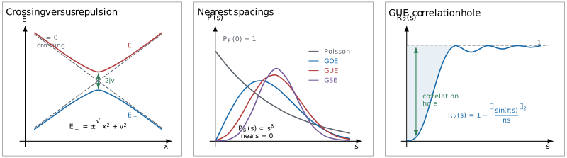
Three complementary views of level repulsion. Left: a symmetry-allowed coupling $v$ converts a crossing into a minimum gap. Center: Poisson statistics remain finite at $s=0$, while the GOE, GUE, and GSE surmises vanish as $s$, $s^2$, and $s^4$. Right: the unfolded GUE two-level correlator $R_2(s)=1-[\sin(\pi s)/(\pi s)]^2$ displays the correlation hole and approaches one at large separation.

Spacing ratios

Define raw consecutive gaps and their symmetrized ratio by

$$\delta_n = E_{n+1}-E_n,$$ $$\widetilde r_n = \frac{ \min(\delta_n,\delta_{n+1}) }{ \max(\delta_n,\delta_{n+1}) }.$$

Because nearby gaps are rescaled by nearly the same smooth density, $\widetilde r_n$ often avoids explicit unfolding. For independent exponential gaps,

$$\left\langle \widetilde r \right\rangle_{\mathrm P} = 2\ln2-1 \simeq 0.38629.$$

Representative large-matrix values are

Statistics	$\left\langle\widetilde r\right\rangle$	Interpretation
Poisson	$0.38629$	exact for independent exponential gaps
GOE	$\simeq0.5307$	large-matrix numerical benchmark
GUE	$\simeq0.5996$	large-matrix numerical benchmark
GSE	$\simeq0.6744$	Kramers pairs counted once

The compact ratio distribution

$$P_\beta(r) = \frac{1}{Z_\beta} \frac{ \left(r+r^2\right)^\beta }{ \left(1+r+r^2\right)^{1+3\beta/2} }, \qquad r\geq0,$$

is itself a small-matrix surmise. Its mean values are close to, but not identical with, the large-matrix numbers above. A ratio average is useful screening evidence; it does not test long-range rigidity.

Two-level correlations and the sine kernel

In the unfolded bulk of the GUE, the large-$N$ process is determinantal with kernel

$$K(s) = \frac{ \sin(\pi s) }{ \pi s }.$$

With mean density one, the normalized two-level correlation function is

$$R_2(s) = 1-K^2(s).$$

Thus

$$R_2(0) = 0, \qquad \lim_{\lvert s\rvert\to\infty} R_2(s) = 1.$$

The missing probability near $s=0$ is the correlation hole. The oscillatory recovery contains more information than a nearest-neighbor histogram.

For the number $n_L$ of unfolded levels in an interval of length $L$, define the number variance

$$\Sigma^2(L) = \left\langle \left( n_L-L \right)^2 \right\rangle.$$

Poisson statistics give

$$\Sigma_{\mathrm P}^2(L) = L.$$

The Wigner–Dyson classes are much more rigid:

$$\Sigma_\beta^2(L) = \frac{2}{\beta\pi^2} \ln L + O(1), \qquad L\gg1.$$

Long-range statistics are more sensitive than ratios to imperfect unfolding, finite bandwidth, missing levels, and slow nonuniversal modes.

One connected GUE form-factor convention is

$$\begin{aligned} K_{\mathrm c}(\tau) &= \int_{-\infty}^{\infty} ds\, e^{-2\pi i\tau s} \\ &\quad\times \left[ \delta(s)+R_2(s)-1 \right]. \end{aligned}$$

It gives

$$K_{\mathrm c}(\tau) = \begin{cases} \lvert\tau\rvert, & \lvert\tau\rvert\leq1, \\ 1, & \lvert\tau\rvert\geq1. \end{cases}$$

The linear ramp and unit plateau follow only with this unfolding and normalization. Finite-temperature filters, disconnected pieces, finite observation windows, and many-body Thouless scales belong to the Many-Body Quantum Chaos Preview.

Wigner–Dyson Classes

Resolve ordinary unitary symmetries first

Suppose a unitary operator $Q$ commutes with $H$. Then

$$\mathcal H = \bigoplus_q \mathcal H_q, \qquad H = \bigoplus_q H_q.$$

Random-matrix statistics must be computed within one irreducible block $H_q$. Momentum, parity, particle number, total spin, point-group representations, and gauge constraints can all produce independent sequences. An antiunitary symmetry may preserve a block, exchange two blocks, or square differently after internal structure is included; checking only the full Hamiltonian is insufficient.

The three bulk classes

After unitary block decomposition, the ordinary bulk classes are:

Altland–Zirnbauer class	Antiunitary structure in the block	Ensemble	$\beta$	Counting rule
AI	$\mathcal T^2=+I$	GOE	$1$	count every nondegenerate level
A	no time-reversal constraint	GUE	$2$	count every level
AII	$\mathcal T^2=-I$	GSE	$4$	count each Kramers pair once

For a spinless Hamiltonian with a basis in which $\mathcal T=K$, time-reversal invariance permits a real symmetric representation and leads to class AI. Breaking the relevant antiunitary symmetry, for example with magnetic flux, gives class A. For half-integer spin with $\mathcal T^2=-I$ and no additional block exchange, Kramers degeneracy leads to class AII.

These are symmetry statements, not statements about whether a material is literally orthogonal, unitary, or symplectic as a vector space. The labels name the transformation groups of the invariant ensemble.

Gaussian versus circular ensembles

Gaussian ensembles describe Hermitian spectra on the real line. For a unitary evolution operator,

$$U \lvert n\rangle = e^{-i\theta_n} \lvert n\rangle,$$

the eigenphases live on a circle. Circular ensembles have joint phase density

$$\mathcal P(\theta_1,\ldots,\theta_N) \propto \prod_{i<j} \left| e^{i\theta_i} - e^{i\theta_j} \right|^\beta.$$

The circular orthogonal, unitary, and symplectic ensembles share their local bulk limits with GOE, GUE, and GSE, respectively. They are natural for Floquet operators and scattering matrices because no artificial spectral edge is introduced. Floquet Operators develops quasienergy kinematics; Floquet Systems Preview treats driven many-body phases and heating.

Crossovers are parameter-dependent

A weak symmetry-breaking perturbation does not instantly replace one finite-size distribution by another. A crossover occurs when its typical matrix element becomes comparable with the local mean spacing. Schematically, if

$$H(\lambda) = H_{\mathrm{AI}} + \lambda V_{\mathrm{A}},$$

then the crossover parameter has the form

$$\Lambda \sim \frac{ \lambda^2 \overline{ \lvert V_{mn}\rvert^2 } }{ \Delta^2 }.$$

The precise coefficient depends on normalization. Reporting only the bare field or flux without $\Delta$, size, and symmetry sector obscures the scaling variable.

Level Repulsion

Vandermonde Jacobian

Diagonalize

$$H = U\Lambda U^{-1}, \qquad \Lambda = \operatorname{diag} (\lambda_1,\ldots,\lambda_N).$$

Changing variables from matrix entries to eigenvalues and eigenvectors produces the Jacobian

$$dH \propto \prod_{i<j} \lvert \lambda_i-\lambda_j \rvert^\beta \prod_i d\lambda_i\, d\mu(U).$$

After integrating over $U$,

$$\begin{aligned} \mathcal P( \lambda_1,\ldots,\lambda_N ) &= \frac{1}{\widetilde Z_{N,\beta}} \exp\!\left[ - \frac{\beta N}{4a^2} \sum_i\lambda_i^2 \right] \\ &\quad\times \prod_{i<j} \lvert \lambda_i-\lambda_j \rvert^\beta. \end{aligned}$$

The Vandermonde factor vanishes when two eigenvalues coincide. In the Coulomb-gas analogy,

$$- \ln\mathcal P = \frac{\beta N}{4a^2} \sum_i\lambda_i^2 - \beta \sum_{i<j} \ln \lvert \lambda_i-\lambda_j \rvert + \text{constant},$$

so eigenvalues behave like charges with logarithmic repulsion in a confining potential. This is an analogy for the joint probability density, not a literal force among energy levels.

Two-level avoided crossings

The local mechanism is visible without the full Jacobian. A real symmetric two-level Hamiltonian can be written

$$H_{\mathrm R} = E_0 I + x\sigma_z + v\sigma_x.$$

Its eigenvalues are

$$E_\pm = E_0 \pm \sqrt{x^2+v^2},$$

and the gap is

$$s \propto \sqrt{x^2+v^2}.$$

Near a degeneracy, the independent splitting coordinates form a two-dimensional vector. A smooth probability density assigns shell volume

$$dP \propto s^{2-1}\,ds,$$

which gives linear repulsion.

For a complex Hermitian two-level block,

$$H_{\mathrm C} = E_0I + x\sigma_x + y\sigma_y + z\sigma_z.$$

There are three splitting coordinates, so

$$dP \propto s^{3-1}\,ds = s^2\,ds.$$

The self-dual quaternionic problem has five independent splitting coordinates after Kramers pairing, giving

$$dP \propto s^{5-1}\,ds = s^4\,ds.$$

Thus the codimension picture and the Vandermonde Jacobian agree:

$$\begin{array}{c|ccc} \text{class} & \mathrm{AI} & \mathrm{A} & \mathrm{AII} \\ \hline \text{splitting coordinates} & 2 & 3 & 5 \\ \text{repulsion exponent} & 1 & 2 & 4 \end{array}$$

When exact crossings remain

Repulsion applies only between levels allowed to hybridize. Levels in different irreducible symmetry sectors can cross because their off-diagonal matrix element vanishes identically. Integrable systems can possess enough conserved structure to support crossings or uncorrelated sequences. Kramers partners remain exactly degenerate when $\mathcal T^2=-I$. Topological or chiral symmetry can pin eigenvalues at a special energy.

An observed crossing therefore asks two separate questions:

1. Is a coupling forbidden by an exact symmetry?
2. If not, is the apparent crossing unresolved because the gap lies below numerical or experimental resolution?

Quantum Chaos

Spectral correspondences

For many generic classically integrable Hamiltonian systems, the Berry–Tabor correspondence predicts Poisson-like unfolded spectra in the semiclassical limit. For systems with a fully chaotic classical limit, the Bohigas–Giannoni–Schmit correspondence predicts the Wigner–Dyson class selected by antiunitary symmetry.

These statements have hypotheses and exceptions. Arithmetic systems, commensurate oscillators, mixed phase space, marginally stable orbits, unresolved discrete symmetries, and finite-energy effects can all alter the result. The Bohigas–Giannoni–Schmit statement is a highly successful universality conjecture, not a theorem covering every chaotic Hamiltonian.

Random-matrix agreement also does not define classical chaos. Unitary quantum evolution preserves the Hilbert-space distance between states evolved by the same operator. Classical sensitivity, periodic-orbit theory, Ehrenfest time, and eigenfunction scarring are developed in Quantum Chaos Preview.

An effective fluctuation theory

A local Hamiltonian may be sparse in a product basis,

$$H_{\mathrm{local}} = \sum_X h_X,$$

with each $h_X$ supported on a small region. A Gaussian random matrix is dense and has no spatial geometry. The comparison is therefore not

$$H_{\mathrm{local}} \simeq H_{\mathrm{RMT}}$$

entry by entry. It is instead

$$\begin{gathered} \text{selected unfolded correlations of } H_{\mathrm{local}} \\ \text{approach the symmetry-compatible} \\ \text{random-matrix correlations in a scale window.} \end{gathered}$$

For a diffusive sample or local many-body system, let $t_{\mathrm{Th}}$ be the exploration or Thouless time,

$$E_{\mathrm{Th}} \sim \frac{\hbar}{t_{\mathrm{Th}}},$$

and let $\Delta$ be the mean level spacing. The dimensionless spectral conductance is

$$g_{\mathrm{Th}} \sim \frac{E_{\mathrm{Th}}}{\Delta}.$$

Random-matrix behavior is expected only below the system-dependent Thouless energy, or after the corresponding time, while microscopic, ballistic, hydrodynamic, and finite-size effects remain outside that window. Quantum Coherence in Conductors owns the competing dephasing, escape, and thermal lengths.

Disorder and localization

In a disordered conductor, spectral statistics provide a compact spatial diagnostic:

Regime	Typical unfolded statistics	Physical reason
Localized	approximately Poisson	distant localized orbitals overlap weakly
Diffusive metal below $E_{\mathrm{Th}}$	Wigner–Dyson	wavefunctions hybridize throughout the coherent sample
Anderson critical point	scale-invariant critical statistics	multifractal states are neither ordinary localized nor metallic

Anderson Localization owns the random lattice Hamiltonian and spatial diagnostics. Mobility Edges owns energy-resolved critical scaling. Spectral statistics should be combined with transfer lengths, participation ratios, transport, or wave-packet spreading because Poisson behavior by itself does not distinguish localization from integrability.

A reproducible evidence ladder

1. Specify the operator. Record the Hamiltonian or unitary, boundary conditions, parameter distribution, size, and numerical precision.
2. Resolve every exact symmetry. Work in one irreducible block and state how antiunitary symmetries act on it.
3. Choose a stationary window. Exclude spectral edges, phase boundaries, protected zero modes, and rapidly varying density unless they are the target.
4. Audit unfolding. Compare several smooth counting functions and report the retained energy fraction.
5. Use short- and long-range statistics. Pair $\widetilde r$ or $P(s)$ with $R_2$, $\Sigma^2$, rigidity, or a connected form factor.
6. Scale size and sample count. Report disorder realizations, block dimensions, confidence intervals, and correlations among bins.
7. Test competing mechanisms. Break or restore a symmetry, move across an integrable point, vary disorder, or compare spatial diagnostics.
8. Limit the claim. Say whether the evidence supports repulsion, random-matrix universality, semiclassical chaos, many-body thermalization, or something stronger.

This ladder prevents the common escalation from “one spacing histogram resembles GOE” to “the system is chaotic and thermalizes.”

Symmetry Classes and Topology

The zero-dimensional tenfold extension

The three Wigner–Dyson classes assume no spectral symmetry that relates $E$ to $-E$. Superconducting and sublattice problems introduce two antiunitary possibilities and one unitary spectral symmetry:

$$\mathcal T H\mathcal T^{-1} = H,$$ $$\mathcal C H\mathcal C^{-1} = -H,$$ $$\mathcal S H\mathcal S^{-1} = -H.$$

Here $\mathcal T$ is time reversal, $\mathcal C$ is Altland–Zirnbauer particle–hole structure, and $\mathcal S$ is chiral symmetry. When both antiunitary symmetries exist, their product gives a chiral symmetry up to a phase. After ordinary commuting unitary symmetries have been resolved, the ten zero-dimensional ensemble classes are:

Class	$\mathcal T^2$	$\mathcal C^2$	$\mathcal S$	Spectral feature
A	$0$	$0$	$0$	unitary Wigner–Dyson bulk
AI	$+1$	$0$	$0$	orthogonal Wigner–Dyson bulk
AII	$-1$	$0$	$0$	symplectic Wigner–Dyson bulk
AIII	$0$	$0$	$1$	chiral pairing about zero
BDI	$+1$	$+1$	$1$	chiral class with real structure
D	$0$	$+1$	$0$	particle–hole pairing; possible unpaired zero mode
DIII	$-1$	$+1$	$1$	Kramers and particle–hole structure
CII	$-1$	$-1$	$1$	chiral symplectic structure
C	$0$	$-1$	$0$	particle–hole pairing with spin structure
CI	$+1$	$-1$	$1$	chiral class with time reversal

A zero means the symmetry is absent, not that its square vanishes. The table classifies allowed matrix constraints. It does not yet assign a spatial topological phase.

In a Bogoliubov–de Gennes Hamiltonian, $\mathcal C$ usually expresses Nambu redundancy:

$$\mathcal C H_{\mathrm{BdG}}(\mathbf k) \mathcal C^{-1} = - H_{\mathrm{BdG}}(-\mathbf k).$$

It should not be confused with an ordinary many-body symmetry that exchanges physical particles and holes while preserving the Hamiltonian.

Special energy requires special statistics

Far from $E=0$, many chiral and superconducting ensembles recover an ordinary Wigner–Dyson bulk class. Near the symmetry point, however, eigenvalues occur in $\pm E$ pairs, exact zero modes may be present, and the density can have a hard edge or class-dependent singularity. The sine kernel and ordinary Wigner surmises are then not the correct complete benchmarks.

The appropriate microscopic kernels depend on:

• the Altland–Zirnbauer class;
• the number of protected zero modes or topological index;
• whether the observation is in the bulk, at a soft edge, or near a hard symmetry point;
• how Kramers and particle–hole partners are counted.

This is why “the histogram is not GOE” is not evidence against universality when the window contains a superconducting zero energy.

From ensemble class to topological phase

To classify a gapped free-fermion phase, one must additionally specify:

$$\begin{gathered} \text{spatial dimension,} \\ \text{bulk gap or mobility gap,} \\ \text{allowed symmetry-preserving deformations,} \\ \text{stable addition of trivial bands.} \end{gathered}$$

Only then does the tenfold pattern lead to dimension-dependent integer, binary, or trivial classifications. Topological Insulators and Topological Superconductors own concrete band invariants and boundary states. Symmetry-Protected Topological Phases owns the interacting distinction between symmetry protection and intrinsic topological order.

Random-matrix theory complements topology by describing finite-volume spectral fluctuations and symmetry-point kernels. It does not replace the bulk invariant, and the Altland–Zirnbauer class alone does not determine one.

Mesoscopic scattering

For a phase-coherent cavity attached to ideal leads, the on-shell scattering matrix satisfies

$$S^\dagger S = I.$$

When the dwell dynamics is sufficiently mixing, circular ensembles provide symmetry-controlled distributions for $S$. Observable conductance, shot noise, and delay times depend additionally on channel number, contact transparency, and transmission eigenvalues. What Is Mesoscopic Physics? gives the scale hierarchy; the scattering formulation should not be reduced to an energy-level histogram.

Common Mistakes

• Mixing momentum, parity, particle-number, spin, or point-group blocks before computing spacings.
• Keeping both members of every Kramers pair and interpreting the resulting zero gaps as clustering.
• Comparing raw energy gaps from a varying density of states with unit-mean formulas.
• Calling a Wigner surmise the exact large-$N$ nearest-neighbor distribution.
• Treating a fitted value of $\langle\widetilde r\rangle$ as proof of long-range rigidity.
• Applying the bulk sine kernel at a spectral edge, mobility edge, or protected zero energy.
• Inferring localization from Poisson statistics without spatial or transport evidence.
• Inferring thermalization or rapid scrambling from level repulsion alone.
• Assuming a local Hamiltonian must look dense and random in its microscopic basis.
• Treating the Bohigas–Giannoni–Schmit correspondence as an unrestricted theorem.
• Using an Altland–Zirnbauer class as though it uniquely specified a topological invariant.
• Calling Bogoliubov–de Gennes particle–hole redundancy ordinary charge-conjugation symmetry.

Exercises

1. Normalize the GOE Wigner surmise

Show that

$$P(s) = \frac{\pi}{2} s e^{-\pi s^2/4}$$

is normalized on $s\geq0$ and has unit mean.

Solution

For $a>0$,

$$\int_0^\infty s e^{-as^2}\,ds = \frac{1}{2a}.$$

With $a=\pi/4$,

$$\int_0^\infty P(s)\,ds = \frac{\pi}{2} \frac{1}{2(\pi/4)} = 1.$$

The mean uses

$$\int_0^\infty s^2e^{-as^2}\,ds = \frac{\sqrt{\pi}}{4a^{3/2}}.$$

Therefore

$$\begin{aligned} \langle s\rangle &= \frac{\pi}{2} \frac{\sqrt{\pi}}{ 4(\pi/4)^{3/2} } \\ &= 1. \end{aligned}$$

Normalization and unit mean fix the two constants in a trial form $As e^{-Bs^2}$.

2. Derive two-level repulsion

For

$$H = \begin{pmatrix} x & v \\ v & -x \end{pmatrix},$$

assume the joint density of $x$ and $v$ is smooth and nonzero at the origin. Derive the small-gap power law.

Solution

The eigenvalues are

$$E_\pm = \pm\sqrt{x^2+v^2},$$

so the gap is

$$g = 2\sqrt{x^2+v^2}.$$

Near the origin, use polar coordinates:

$$dx\,dv = r\,dr\,d\phi.$$

Because $g=2r$,

$$dP \propto r\,dr \propto g\,dg.$$

Hence

$$P(g) \propto g$$

at small $g$, the $\beta=1$ repulsion law. If $v$ is forced to zero by a symmetry, the radial argument collapses and an exact crossing at $x=0$ is allowed.

3. Unfold a nonuniform spectrum

Suppose three positive levels are

$$E_1=E_0, \qquad E_2=4E_0, \qquad E_3=9E_0,$$

and the smooth counting function is

$$\overline N(E) = \sqrt{\frac{E}{E_0}}.$$

Find the raw and unfolded gaps.

Solution

The raw gaps are

$$\delta E_1 = 3E_0, \qquad \delta E_2 = 5E_0.$$

The unfolded levels are

$$\varepsilon_1=1, \qquad \varepsilon_2=2, \qquad \varepsilon_3=3.$$

Thus

$$s_1=s_2=1.$$

The increasing raw gaps came entirely from the decreasing smooth density. Treating them as changing correlations would be a false inference.

4. Derive the Poisson ratio mean

Let $x$ and $y$ be independent exponential gaps with density $e^{-x}$ for $x\geq0$. Show that

$$\widetilde r = \frac{\min(x,y)}{\max(x,y)}$$

has mean $2\ln2-1$.

Solution

By symmetry, integrate over $0\leq x\leq y$ and double:

$$\left\langle \widetilde r \right\rangle = 2 \int_0^\infty dy \int_0^y dx\, \frac{x}{y} e^{-x-y}.$$

Set $x=ry$, so $dx=y\,dr$:

$$\left\langle \widetilde r \right\rangle = 2 \int_0^1 dr\,r \int_0^\infty dy\, y e^{-(1+r)y}.$$

The inner integral is $1/(1+r)^2$, hence

$$\begin{aligned} \left\langle \widetilde r \right\rangle &= 2 \int_0^1 \frac{r}{(1+r)^2}\,dr \\ &= 2\ln2-1 \\ &\simeq 0.38629. \end{aligned}$$

5. Compare long-range rigidity

At $L=20$, compare the Poisson number variance with the leading logarithmic term for the GUE.

Solution

Poisson statistics give

$$\Sigma_{\mathrm P}^2(20) = 20.$$

For $\beta=2$, the leading growing term is

$$\frac{1}{\pi^2} \ln20 \simeq 0.3035.$$

The omitted $O(1)$ constant is numerically important at $L=20$, so $0.3035$ is not a precision prediction for the full GUE variance. The robust comparison is linear growth versus logarithmic growth.

6. Count Kramers pairs correctly

A finite class-AII spectrum is listed as

$$E_1,E_1,E_2,E_2,E_3,E_3.$$

What goes wrong if all six entries are used in a nearest-neighbor histogram, and what sequence should be analyzed?

Solution

Keeping all entries produces gaps

$$0,\, E_2-E_1,\, 0,\, E_3-E_2,\, 0.$$

The delta weight at zero is the exact Kramers degeneracy, not a failure of symplectic repulsion. Count each pair once and analyze

$$E_1,E_2,E_3,\ldots$$

within one otherwise irreducible block. The expected small-spacing law is then

$$P(s) \propto s^4.$$

7. Classify two matrix problems

Classify the following zero-dimensional Hamiltonians:

1. a real symmetric spinless Hamiltonian with $\mathcal T=K$ and no spectral symmetry;
2. a Bogoliubov–de Gennes Hamiltonian with $\mathcal C^2=+I$, no time reversal, and no chiral symmetry.

Does either class label alone determine a three-dimensional topological invariant?

Solution

The first problem has

$$\mathcal T^2 = +I$$

and belongs to class AI, whose ordinary bulk ensemble is GOE.

The second has particle–hole structure with positive square and belongs to class D.

Neither label alone determines a three-dimensional invariant. One must specify spatial dimension, the type of bulk or mobility gap, stabilization, and the allowed symmetry-preserving deformations. Interactions can further change a free-fermion classification.

8. Audit a chaos claim

A paper pools all parity and momentum sectors of a spin chain, fits one bulk spacing histogram to the GOE Wigner surmise, and concludes that the model is chaotic, thermalizing, and rapidly scrambling. List at least eight missing checks or distinctions.

Solution

A defensible audit should require:

1. separate irreducible momentum and parity blocks;
2. treatment of particle number, total spin, inversion, and accidental degeneracies;
3. the action and square of time reversal within the chosen block;
4. exclusion of spectral edges and a declared energy-density window;
5. unfolding stability or an adjacent-gap-ratio cross-check;
6. long-range statistics such as number variance or a connected form factor;
7. system-size and parameter scaling through nearby integrable regimes;
8. sample counts, bin correlations, and uncertainty estimates;
9. an ETH matrix-element or eigenstate test before claiming thermalization;
10. an operator-spreading or OTOC diagnostic before claiming rapid scrambling;
11. a Thouless-time analysis before asserting random-matrix behavior at every scale;
12. controls for mixed phases, scars, fragmentation, and other atypical subspaces.

The reported histogram may support local repulsion after reanalysis. It cannot, by itself, establish the stronger dynamical claims.

Connections

• Quantum Chaos Preview develops classical sensitivity, semiclassical periodic-orbit structure, Ehrenfest time, eigenfunction scars, and the Bohigas–Giannoni–Schmit bridge.
• Many-Body Quantum Chaos Preview owns local-system spectral workflows, Thouless and Heisenberg times, ETH, many-body form factors, and limits on chaos claims.
• Symmetry Classification Preview derives the $\mathcal T$, $\mathcal C$, and $\mathcal S$ vocabulary underlying the ten Altland–Zirnbauer classes.
• Anderson Localization connects Poisson, Wigner–Dyson, and critical spectra to localized, metallic, and multifractal wavefunctions.
• Mobility Edges owns energy-resolved finite-size scaling and explains why critical statistics are neither ordinary Poisson nor metallic Wigner–Dyson.
• Finite-Size Scaling in Numerics develops crossing fits, irrelevant corrections, covariance-aware uncertainties, and collapse audits.
• Quantum Coherence in Conductors explains the dephasing, thermal, and escape scales that delimit mesoscopic universality.
• Topological Insulators and Topological Superconductors own dimension-dependent invariants and boundary states.
• Floquet Systems Preview applies circular-ensemble ideas to quasienergies while separating spectral correlations from heating and phase structure.

References

1. E. P. Wigner, “Characteristic Vectors of Bordered Matrices With Infinite Dimensions,” Annals of Mathematics 62, 548–564 (1955), doi:10.2307/1970079. Introduces statistical matrix methods for complex spectra and the small-matrix spacing approximation.
2. F. J. Dyson, “Statistical Theory of the Energy Levels of Complex Systems. I,” Journal of Mathematical Physics 3, 140–156 (1962), doi:10.1063/1.1703773. Develops invariant eigenvalue ensembles and the logarithmic-gas structure.
3. F. J. Dyson, “The Threefold Way: Algebraic Structure of Symmetry Groups and Ensembles in Quantum Mechanics,” Journal of Mathematical Physics 3, 1199–1215 (1962), doi:10.1063/1.1703863. Establishes the orthogonal, unitary, and symplectic symmetry trichotomy.
4. M. V. Berry and M. Tabor, “Level Clustering in the Regular Spectrum,” Proceedings of the Royal Society A 356, 375–394 (1977), doi:10.1098/rspa.1977.0140. Formulates the semiclassical Poisson correspondence for generic integrable systems.
5. O. Bohigas, M.-J. Giannoni, and C. Schmit, “Characterization of Chaotic Quantum Spectra and Universality of Level Fluctuation Laws,” Physical Review Letters 52, 1–4 (1984), doi:10.1103/PhysRevLett.52.1. States the spectral-universality correspondence for classically chaotic systems.
6. K. B. Efetov, “Supersymmetry and Theory of Disordered Metals,” Advances in Physics 32, 53–127 (1983), doi:10.1080/00018738300101531. Connects disordered conductors, nonlinear sigma models, and zero-dimensional random-matrix limits.
7. A. Altland and M. R. Zirnbauer, “Nonstandard Symmetry Classes in Mesoscopic Normal-Superconducting Hybrid Structures,” Physical Review B 55, 1142–1161 (1997), doi:10.1103/PhysRevB.55.1142. Completes the tenfold ensemble classification for normal and Bogoliubov–de Gennes systems.
8. C. W. J. Beenakker, “Random-Matrix Theory of Quantum Transport,” Reviews of Modern Physics 69, 731–808 (1997), doi:10.1103/RevModPhys.69.731. Reviews circular ensembles, transmission eigenvalues, and mesoscopic transport.
9. T. Guhr, A. Müller-Groeling, and H. A. Weidenmüller, “Random-Matrix Theories in Quantum Physics: Common Concepts,” Physics Reports 299, 189–425 (1998), doi:10.1016/S0370-1573(97)00088-4. Gives a broad account of correlation functions, universality, and physical applications.
10. A. D. Mirlin, “Statistics of Energy Levels and Eigenfunctions in Disordered Systems,” Physics Reports 326, 259–382 (2000), doi:10.1016/S0370-1573(99)00091-5. Develops the relation among spectral statistics, eigenfunctions, diffusion, and localization.
11. J. J. M. Verbaarschot and T. Wettig, “Random Matrix Theory and Chiral Symmetry in QCD,” Annual Review of Nuclear and Particle Science 50, 343–410 (2000), doi:10.1146/annurev.nucl.50.1.343. Explains hard-edge universality, chiral ensembles, and topological zero modes in a mature application.
12. L. Erdős, B. Schlein, and H.-T. Yau, “Universality of Random Matrices and Local Relaxation Flow,” Inventiones Mathematicae 185, 75–119 (2011), doi:10.1007/s00222-010-0302-7. Proves broad local universality for Wigner matrices under controlled hypotheses.
13. Y. Y. Atas, E. Bogomolny, O. Giraud, and G. Roux, “Distribution of the Ratio of Consecutive Level Spacings in Random Matrix Ensembles,” Physical Review Letters 110, 084101 (2013), doi:10.1103/PhysRevLett.110.084101. Derives practical spacing-ratio surmises and benchmark means.
14. F. Evers and A. D. Mirlin, “Anderson Transitions,” Reviews of Modern Physics 80, 1355–1417 (2008), doi:10.1103/RevModPhys.80.1355. Reviews metallic, localized, and critical spectral statistics across localization classes.
15. A. Kitaev, “Periodic Table for Topological Insulators and Superconductors,” AIP Conference Proceedings 1134, 22–30 (2009), doi:10.1063/1.3149495. Connects symmetry classes to dimension-dependent stable topological classifications.
16. S. Ryu, A. P. Schnyder, A. Furusaki, and A. W. W. Ludwig, “Topological Insulators and Superconductors: Tenfold Way and Dimensional Hierarchy,” New Journal of Physics 12, 065010 (2010), doi:10.1088/1367-2630/12/6/065010. Develops the dimensional hierarchy and boundary interpretation of the tenfold classes.

Further Reading

• M. L. Mehta, Random Matrices, 3rd ed., Elsevier, 2004. A standard technical reference for invariant ensembles and correlation functions.
• F. Haake, Quantum Signatures of Chaos, 3rd ed., Springer, 2010, doi:10.1007/978-3-642-05428-0. A systematic bridge from classical chaos to spectral and eigenfunction diagnostics.
• G. Akemann, J. Baik, and P. Di Francesco, eds., The Oxford Handbook of Random Matrix Theory, Oxford University Press, 2011, doi:10.1093/oxfordhb/9780198744191.001.0001. A broad reference spanning exact methods, universality, and applications.